

Sector 7 contains a scatter plot, or a Poincare plot. With respect to HRV, this is a graphical method for displaying the relationship between successive R-R intervals (cardiac cycles). When constructing this plot, the position of each point is determined by two coordinates: on the ordinate axis (vertical axis) – the duration of the RRi interval, on the abscissa axis (horizontal axis) – the preceding one, RRi-1 (Fig. 2.23a). By default, the sector immediately displays plots for all stages (Fig. 2.23a). On the left side, a column is displayed with the names of all these stages (in our example, Stressonika), marked with the corresponding color (as are the plots in the sector) and with a window where the activation mark is set (Fig. 2.23b). You can visualize the stages that interest you by removing the activation mark or setting it. You can clear the plot field at once by clicking on the cross in the upper left corner (Fig. 2.23b). The result of this action is shown in Fig. 2.23c.
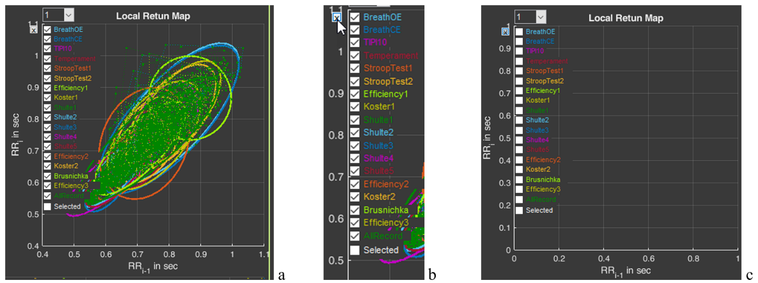
Figure 2.23. HRV Poincare plot in sector 7 and the ability to control the image on the plot (explanations in the text)
Activate the Poincare plot on the graph only for the “BreathOE” stage (Fig. 2.24a). We remember that the plot scale can be controlled using the functional icons (Fig. 2.24b). It is possible to activate plots not for one, but for several stages for comparison (Fig. 2.24c).
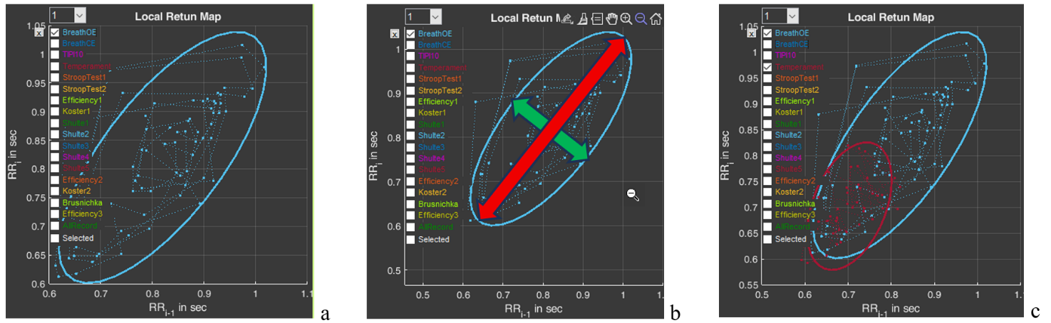
Figure 2.24. HRV Poincare plot for the “BreathOE” stage (explanations in the text)
Now a few words about the scatter plot. The HRV Poincare plot is a visual representation of the integral picture of HRV, which makes it possible to assess the activity of regulatory systems by the shape of the “cloud” of points: a compressed cloud may indicate low variability; by the location of the cloud one can judge HR (we remind you that the smaller the RR-interval value, the higher the HR, and vice versa); the symmetrical shape of the oval outlining the cloud and its optimal form indicate a balance of the autonomic nervous system; significant outliers of points beyond the main cloud most often indicate a significant rhythm disturbance.
The cloud itself is assessed by the shape of the oval drawn around it and by the values of SD1 (the width of the cloud – the green arrow), SD2 (the length of the cloud – the red arrow) (Fig. 2.24b) and their ratio SD1/SD2 (see Table 1).
Using the plot, it is possible to: trace how the body adapts to stress (in the case of Stressonika, this is cognitive stress); assess the balance between the sympathetic and parasympathetic divisions of the autonomic nervous system; track how HRV changes over time under the influence of certain effects, for example, breathing practices.
And one more function of sector 7 is the window with the number 1 (Fig. 2.254a). The number can be changed by activating this window (Fig. 2.25b). For example, we selected the number 5 (Fig. 2.25c). As can be seen, the shape and position of the cloud have changed. This is because on the abscissa axis we selected not the value RRi-1, but the value RRi-5. This function is needed to search for an autocorrelation dependence. But this is already for very advanced scientific research work.
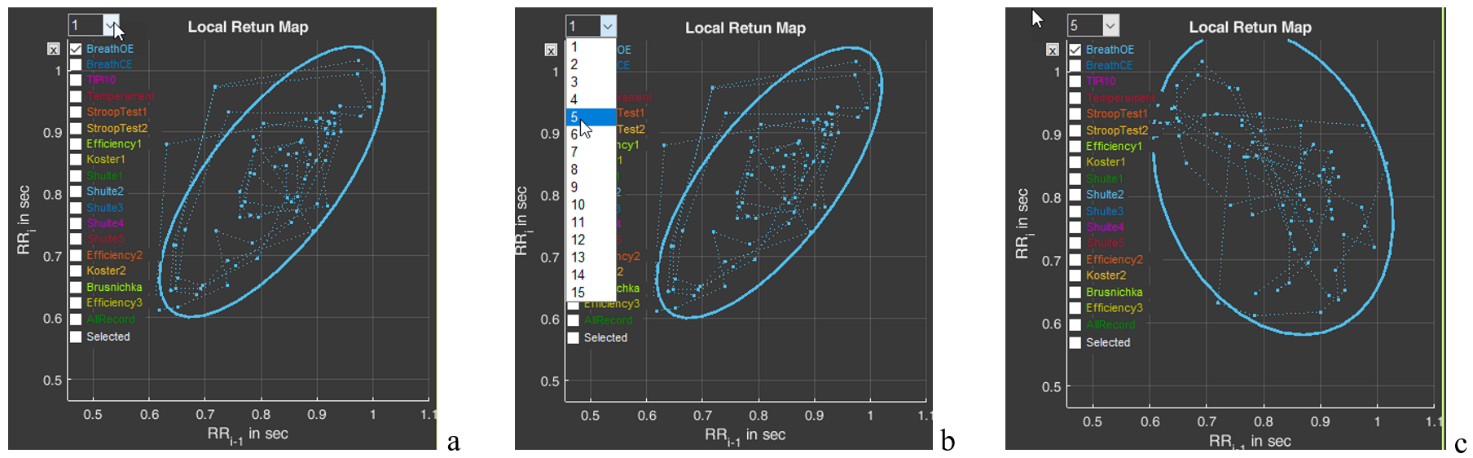
Figure 2.25. Search for an autocorrelation dependence using the “BreathOE” stage as an example (explanations in the text)
Please note that two line segments extend from each point of the diagram, forming an angle. This is the same angle that is taken into account when constructing the histogram we described above (Fig. 2.22).