Stressonika - Guide for Working with raw ECG data

Introduction

You (your company, university, department, etc.) have purchased the CleverPoint Stressonika product for testing persons (employees, clients, research participants, etc.). Working with Stressonika without working with the CleverntView software product is possible, but it will not be as effective, will not be insured against erroneous conclusions, will not provide an opportunity for generalization, statistical data processing, retrospective analysis, and a scientific approach to the results obtained from the studies performed.

Why does Stressonika work better with CleverView?

First, CleverView allows you to visualize the obtained bioelectric signals in the form of an electrocardiogram (ECG), cardiointervalogram (CIG), electroencephalogram (EEG), electromyogram (EMG) and other data both for the entire observation period and for the period of testing that is of interest to you. This is extremely important, as it helps to avoid erroneous interpretation of the report if the sensors are applied incorrectly, the recording is overloaded with artifacts related to technical or biological interference. In addition, an ECG even in a single lead can make it possible to see gross deviations of the heart rhythm and to refer a person in time to a specialist for professional examination.

Second, the visual coverage of the cardiointervalogram, reflecting fluctuations of the RR interval, during the test in Stressonika will allow you to form a picture of the respondent’s autonomic status and assess the mobility of the regulation processes of the psychophysiological state. In combination with the data of the automatic report, this will make it possible not only to comment on the results obtained more weightily and argumentatively, but also to illustrate your conclusions with the help of graphs built in ClevertView. This form of communication makes an impression and makes a person think about themselves not only as a personality, but also as a biological subject whose functioning sometimes needs targeted adjustment.

Third, CleverView allows you to obtain digitized data on the dynamics of RR intervals and heart rate variability (HRV) indices. These values can be stored in accessible databases, collected, systematized, generalized, and used to create your own card index for special groups of respondents. Over time, this work on the evidential basis of your views will give significant weight to your consultations when working with people who come for testing.

Fourth, CleverView contains a modern set of mathematical methods for data processing which, when used skillfully, expand the arsenal of skills of a consultant and/or researcher working with Stressonika.

Fifth, skillful use of scientific approaches in data processing and presentation will increase both your internal self-esteem and the level of trust when communicating with a person who has come to you with their psychological or somatic problems.

If our arguments for the need to master CleverView were sufficiently convincing, we suggest that you familiarize yourself with this manual for working with our software application for Stressonika.

We find the CleverView program shortcut, click it, and begin to study and work.

Success and good luck!

General points

Let us start with general points which you, using our example, can apply in your work, or which you will encounter on any CleverView page.

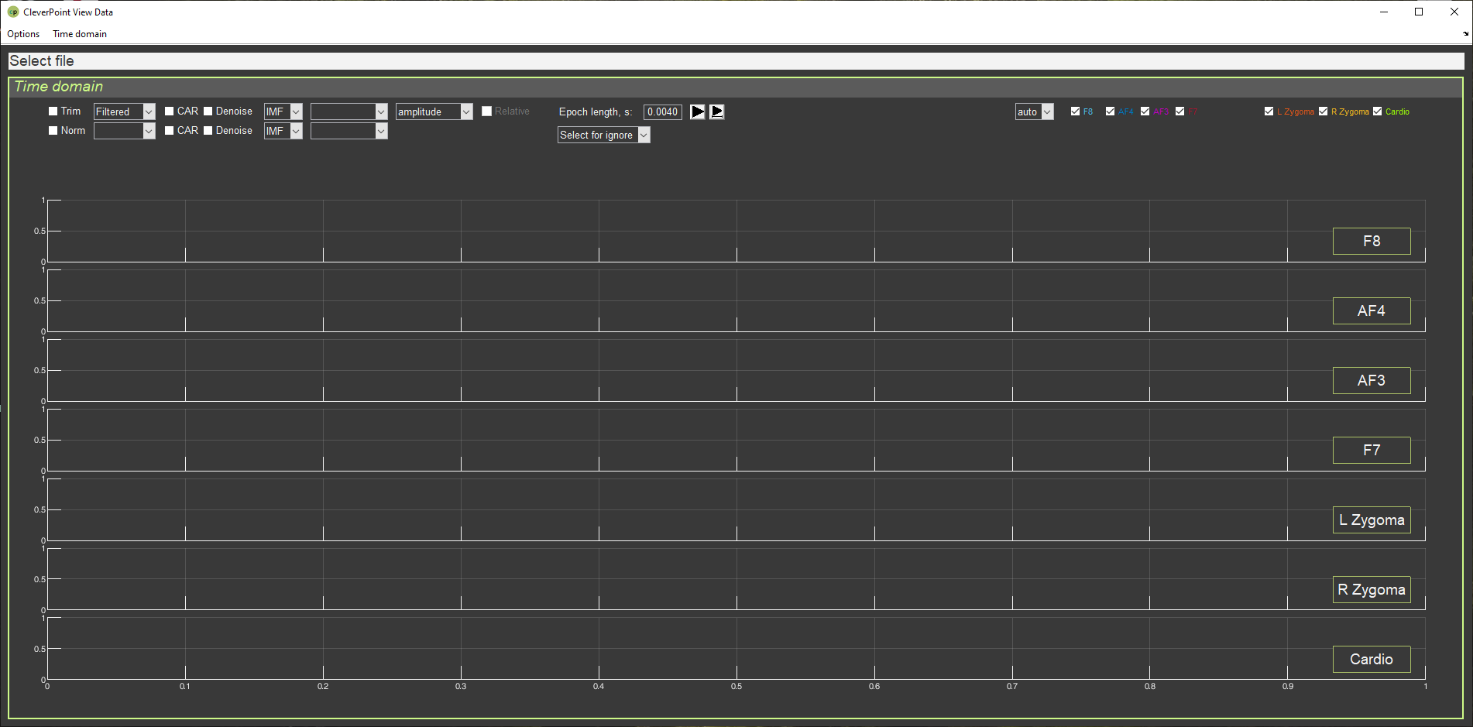
If you have already clicked on the CleverView shortcut on your desktop, the start page “Time domain” (Fig. 1.1) should already have opened.

Figure 1.1. CleverView start page.

We recommend studying this manual in parallel with the CleverView program running (active). At first, do this step by step together with the manual; then, as you become familiar with working in the program, selectively, with those chapters that you wish to study additionally.

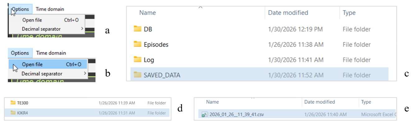
Now let us load the file with the data of the person who interests you. Click on the “Options” window in the upper left corner of the screen (Fig. 1.2.a), then on “Open file” (Fig. 1.2.b), and you will get to the navigation window, in the “SAVED DATA” folder of which the data of your recordings are stored (Fig. 1.2.c). Files are written to the “SAVED DATA” folder automatically and are stored in a folder identified by the respondent’s code and the sequential number of the recording (Fig. 1.2.d). In the respondent’s own folder, the file with the *.csv extension (where instead of * is the date and time of the recording) is the very file intended for loading into CleverView (Fig. 1.2.c).

Figure 1.2. Step-by-step search for the required file to load.

Double-click the file with the *.csv extension and wait. We immediately make a reservation,
as this point is extremely important: during the internal operation of the program in CleverView – whether it is loading a file, a page, or mathematical processing of raw data – the Select file line (see Fig. 1.1) will be highlighted in red (Fig. 1.3).

Figure 1.3. Appearance of the window with the name of the selected file during the internal operation of the CleverView program.

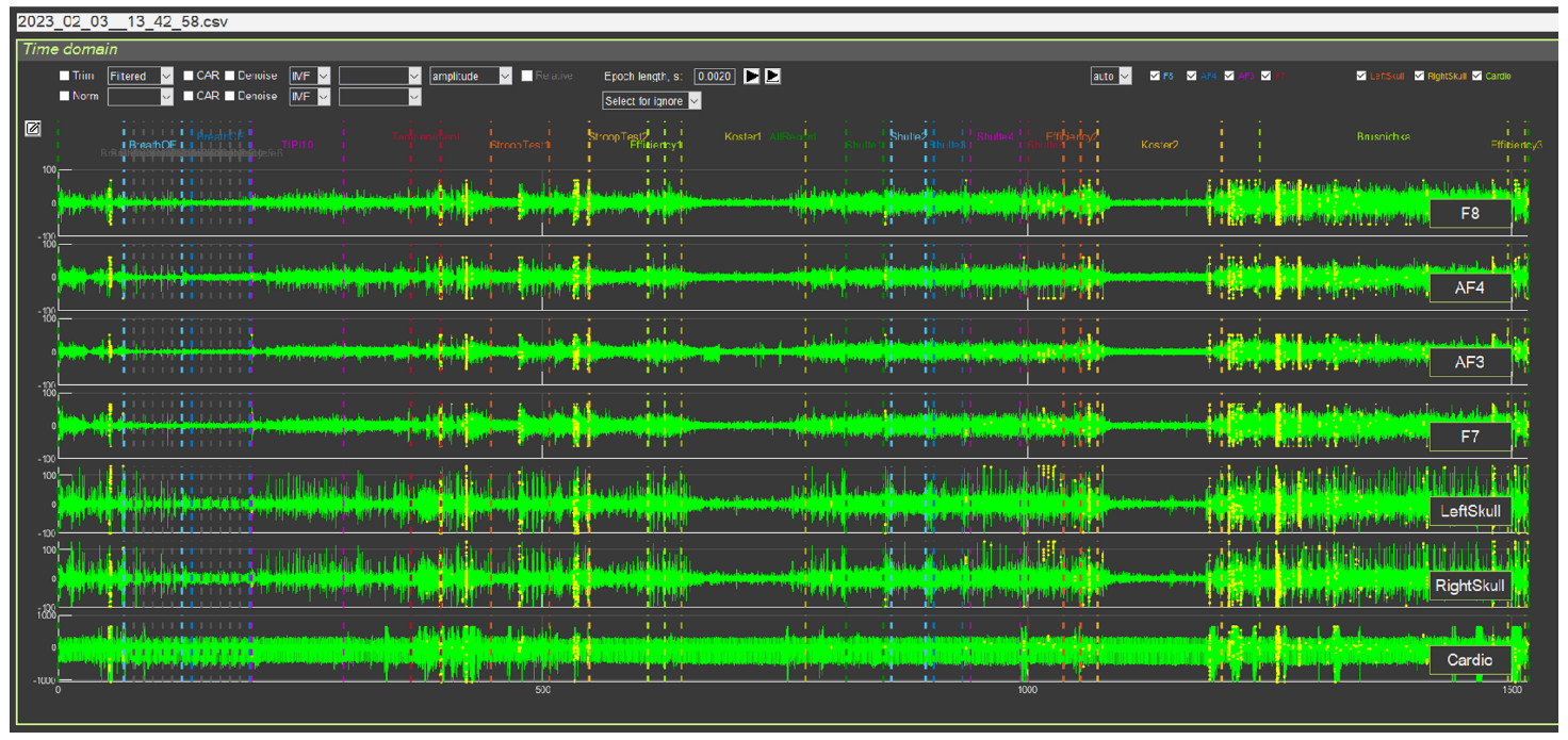
When the required file is loaded, the start page will display EEG curves (leads F8, AF4, AF3 and F7, located in the frontal regions on the facial pad), EMG (L and R Zygoma, located in the area of the zygomatic bone) and ECG (Cardio). The screen will show curves for the entire period of testing in Stressonika, and this is at least 20 minutes. Therefore, for each lead you will see dense “pickets” of bioelectric curves with which you will have to work (Fig. 1.4).

Figure 1.4. CleverView start page with a loaded file

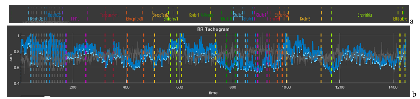
The “Time domain” page is intended for working with the raw data of the signals displayed on it. We immediately draw your attention to the upper part of the screen, above the EEG curve in lead F8 (Fig. 1.5). In this place all stages of testing in Stressonika are indicated. Note the color designation of each stage, which will be repeated on every CleverView page. Each stage is also bounded by vertical dashed lines of the corresponding color, which allows, if necessary, to select the segment that interests us on the graphs.

Figure 1.5. Part of the screen indicating the stages of testing in Stressonika

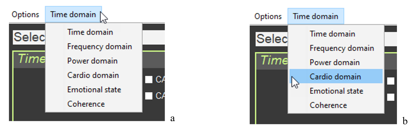
For an overall picture of the psycho-emotional state of a person who has been tested, and for illustrative help during a consultation, the “Cardio domain” page is the most suitable. We will turn to it to consider the most general points, and we will return to “Time domain” in the relevant chapter of the manual. Click on the “Time domain” window in the upper left corner of the screen (Fig. 1.6.a), select the “Cardio domain” tab (Fig. 1.6.b), and click once.

Figure 1.6. Step-by-step search for the page to load, using “Cardio domain” as an example

Wait for the screen to change and for the highlighting of the window with the name of the selected file in red to end. The structure of the “Cardio domain” page is shown in Figure 1.7.

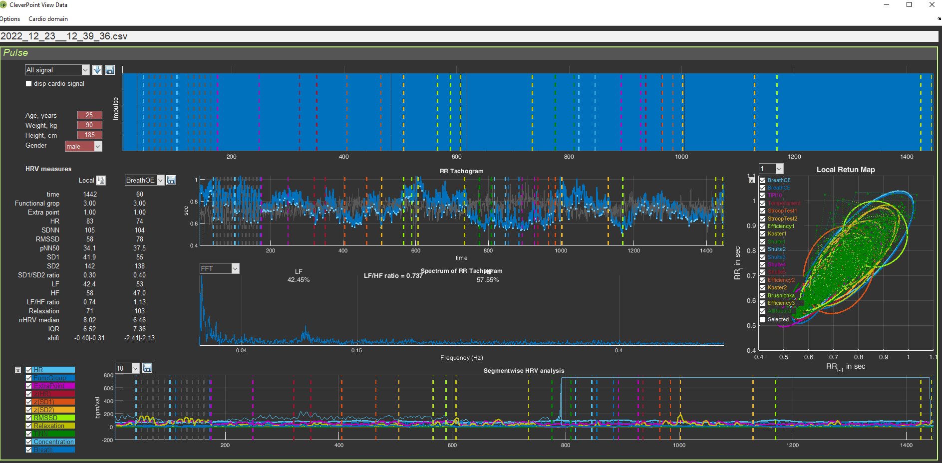
Figure 1.7. “Cardio Domain” page for a loaded file with raw data

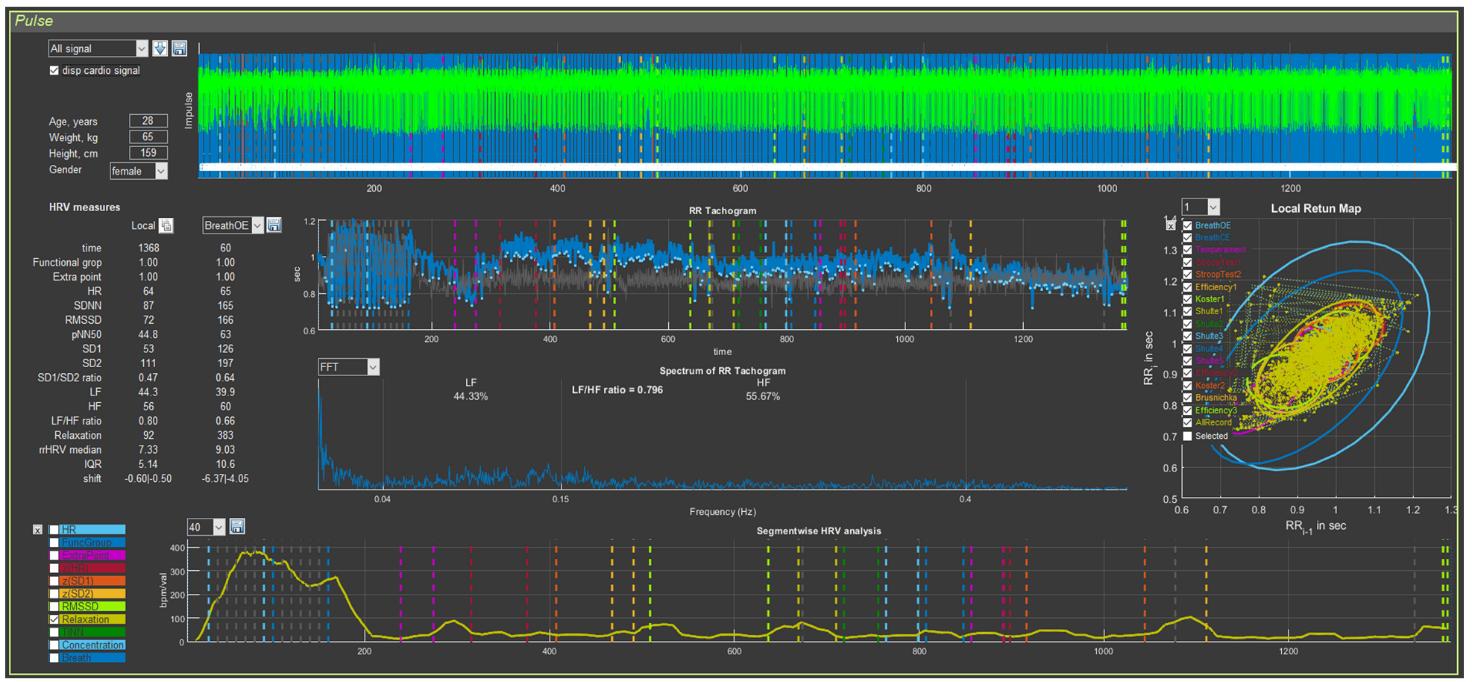
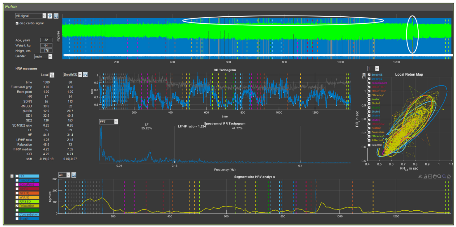
On the “Cardio domain” page, 5 graphs and digital data related to heart rate variability (HRV) are visualized. We will conduct a detailed analysis of this page in the next chapter. For now, we simply get used to it and will examine a few more general points: graph control and orientation by the stages of testing.

Let us return to Figure 6 and pay attention to the vertical bars on each of the graphs, and to the labels and ovals on the “cloud” of points on the graph on the right on the “Cardio Domain” page. Everything is the same as on the “Time domain” page (confirming what has already been said: the same system for marking the stages of testing in Stressonika will be preserved on other pages).

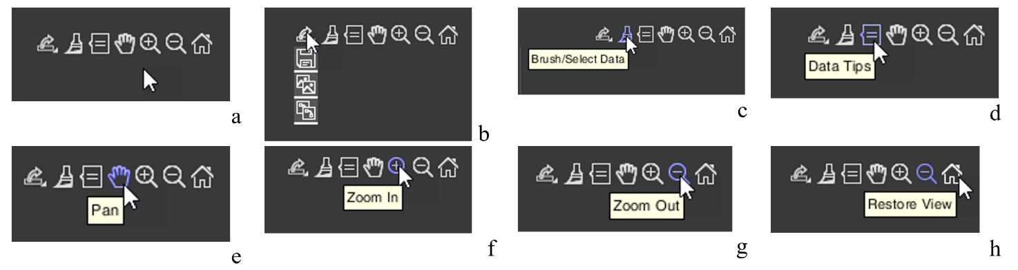
Now let us move the cursor to the upper right of one of the graphs… Icons appear that allow you to control the graph image (Fig. 1.8.a). Let us get acquainted with them. Examples of their use will be given in the next chapter.

Figure 1.8. Icons for controlling the graph image (explanations in the text)

Graph image saving icon (Fig. 1.8.b). Clicking the corresponding pictogram will give you the opportunity to save the graph image where you want, and under the name you specify.
These are typical actions for programs built into Windows.

Icon for color highlighting of a segment of the graph – “Brush/Select Data” (Fig. 1.8.c). This function can be useful for creating an illustration in which you want to emphasize what is seen, described, or commented on.

Icon that allows you to place a marker on the graph – “Data Tips” (Fig. 1.8.d). Activating this icon gives you the opportunity to find out the exact coordinates of a point on the curve, with a window displaying the data of this point along the x- and y-axes. The coordinates are different for each graph. Their description will be provided in the chapters where these graphs will be described. Examples of using this icon will also be given there. It is possible to display data not for one point, but for several. This possibility opens when holding down the “alt” key on the keyboard.

Hand icon – “Pan” (Fig. 1.8.e) will allow you, while holding down the left mouse button on the graph with the corresponding cursor, to scroll the graph to the right or left, or shift it up or down.

The icon with the “+” sign – “Zoom In” (Fig. 1.8.f) opens the function of enlarging the graph horizontally or vertically; the icon with the “-” sign – “Zoom Out” (Fig. 1.8.g) – reduces it.

The last icon in the form of a house – “Restore View” (Fig. 1.8.h) – restores the original appearance of the graph after your actions with it. This function is very useful, and you will be convinced of this when you begin to routinely work with CleverView.

The general points are described. Now you can proceed to studying the individual pages of our CleverView software product.

Cardio domain

Let us begin with the “Cardio domain” page. This page is a visual illustration of the respondent’s general psychophysiological state. When you gain experience and have “looked at” images of this page from different people, you will be able, just by looking at these graphs and numbers, to build your dialogue with the respondent in a reasoned way, emphasizing the report data with objective graphs of a person’s physiological response to one or another task in Stressonika.

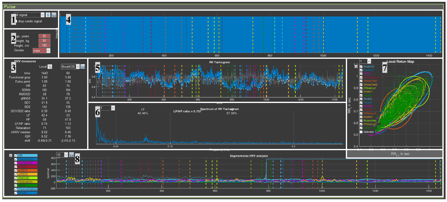
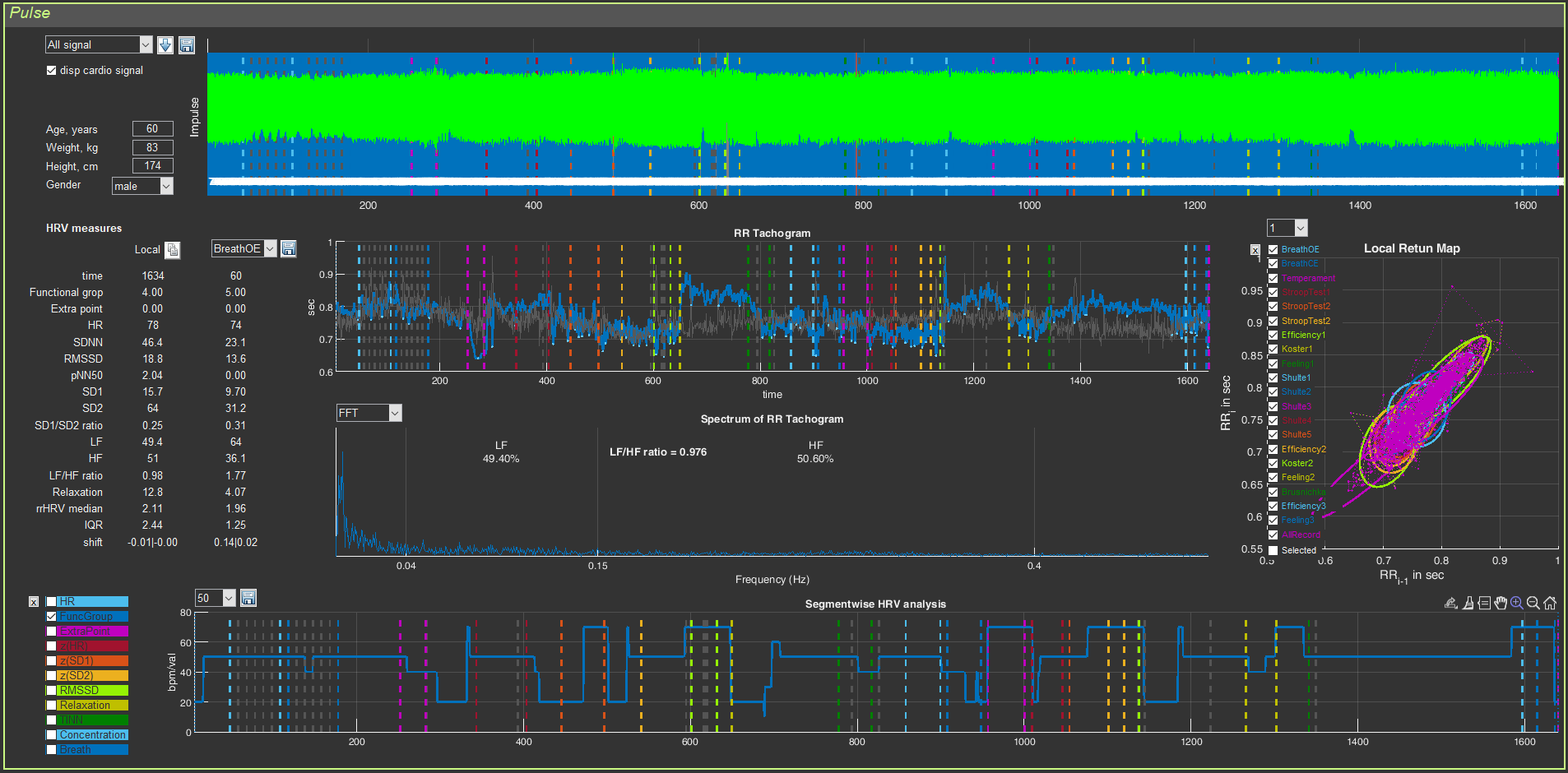
There is another important point that should be highlighted separately: the visual series of this page will immediately indicate to you how well the data collection was carried out (on this page, as we have already indicated, 5 graphs and digital data related to HRV are visualized, which is based on the ECG curve). Examples of poor-quality recordings or recordings with non-critical defects and how to react to this, we will consider below. For now, let us analyze the “Cardio domain” page using the example of a good ECG recording. For the convenience of studying work with this page, we divided it into 8 sectors (Fig. 2.1).

Figure 2.1. “Cardio Domain” page for a loaded file with raw data (explanations in the text)

Highlighting the sectors is an extremely conditional measure, since they are interconnected and changing one can affect another; therefore, the illustration of our actions will be such that you can see these interconnections.

Now, perhaps, we can consider each sector in more detail.

Sector. 1

Sector 1 allows: 1) to display the ECG curve in sector 4, 2) to control visualization of the stages of the study, 3) to save RR interval data in Excel, and 4) to recalculate HRV measures on the ECG segment you selected.

Sector. 1.1

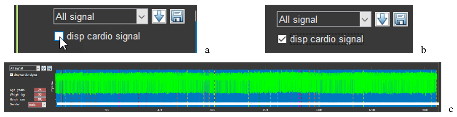
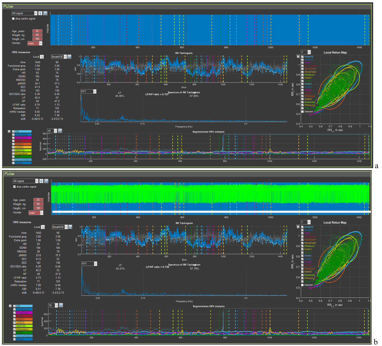
Let us begin by displaying the ECG curve in sector 4: move the cursor to the “disp cardio signal” window (Fig. 2.2a), put a mark in it (Fig. 2.2b), wait a little (remembering the red-colored line with the name of the activated file), and obtain the green ECG curve (Fig. 2.2c).

Figure 2.2. Sequence of actions to activate the ECG curve

In the window for controlling the visualization of the stages of the study, “All signal” is selected (Fig. 2.2a,b), which means that in sector 4 the ECG complexes will be displayed over the markers of the found R waves for the entire examination time. If another stage is activated, then the picture in sector 4 will be different (see below).

Sector. 1.2

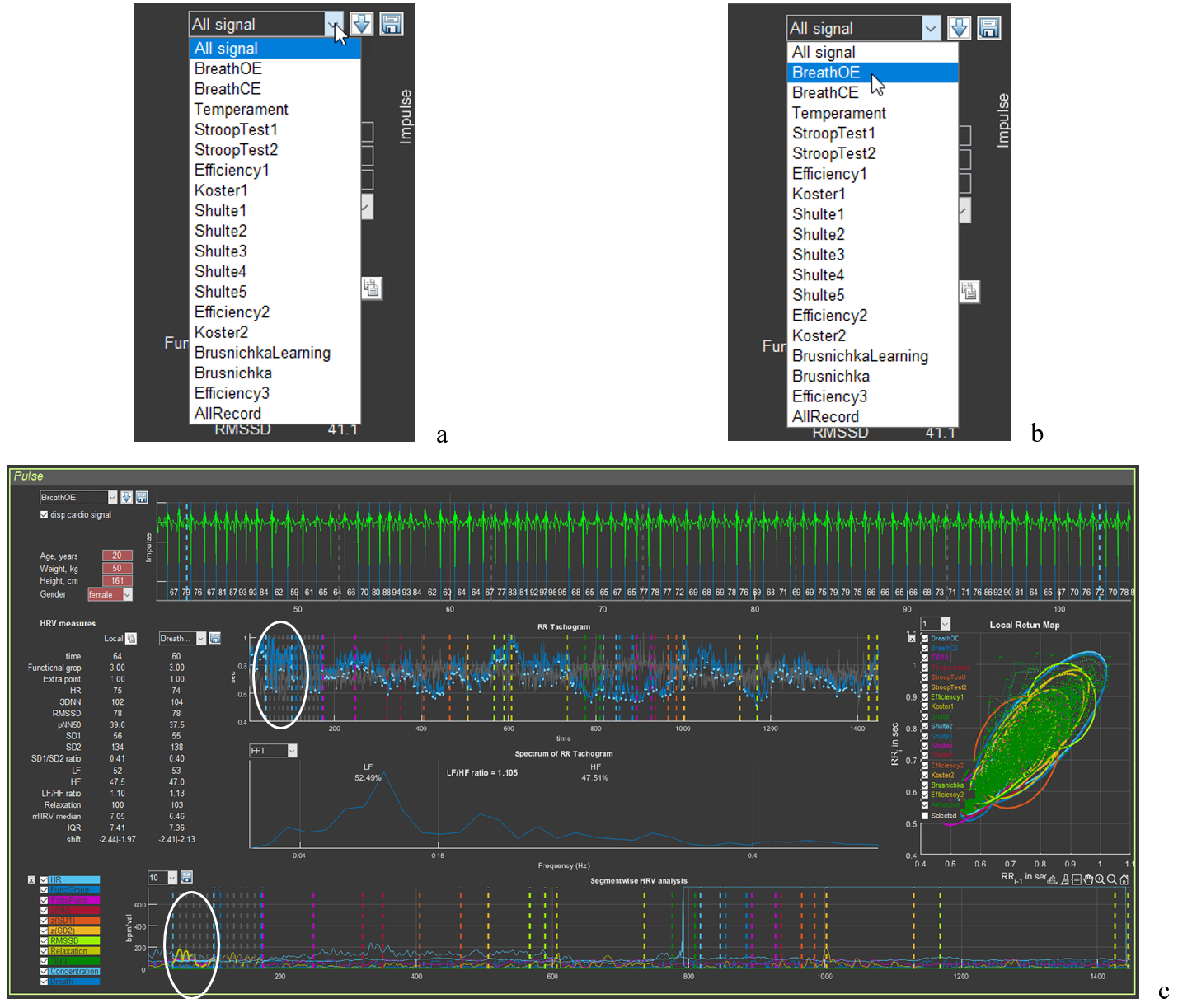
Control of the visualization of the stages of the study is shown in Figure 2.3.

Figure 2.3. Sequence of actions for visualizing the stages of the study (explanations in the text)

Move the cursor to the “button” for activating the list of stages of the study (Fig. 2.3a), select the stage you need (in our example, this is slow breathing with open eyes – BreathOE) (Fig. 2.3b), click on the stage name, and wait; the resulting outcome is shown in Fig. 2.3c. Pay attention to sectors 3, 4, 5, 6, and 8.

In sector 3 under the “Local” label, the numbers corresponding to the HRV measures written in the first column will correspond to the duration of the ECG curve placed in the sector 4 window.

In sector 4, only the ECG segment corresponding to the BreathOE stage is presented (between the vertical dashed lines of the color corresponding to the stage at the beginning and at the end of the sector window). We note immediately that the ECG is positioned with the R wave downward; the blue lines are the R waves detected by the program. When “All signal” is activated, they produce that blue background of the sector (Fig. 2.1), provided that practically all R waves are recorded.

In sectors 5 and 8, the BreathOE stage is highlighted on the curves with a thicker line (we have highlighted it with a white oval).

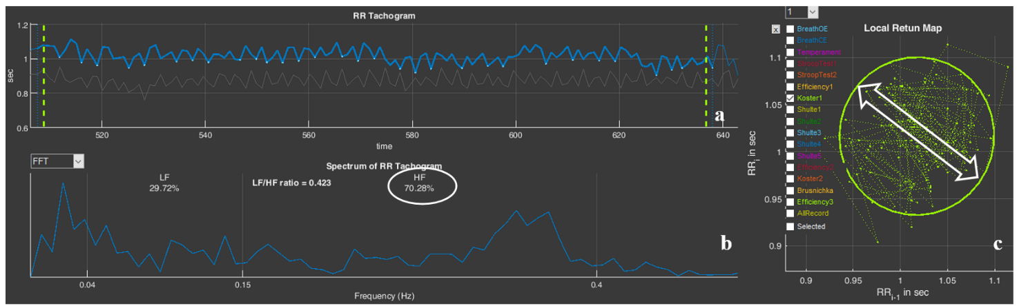
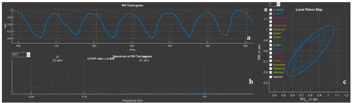
In sector 6, a spectrogram is presented that reflects the dynamics of changes in RR intervals during the period of slow breathing with open eyes – BreathOE.

Sector. 1.3

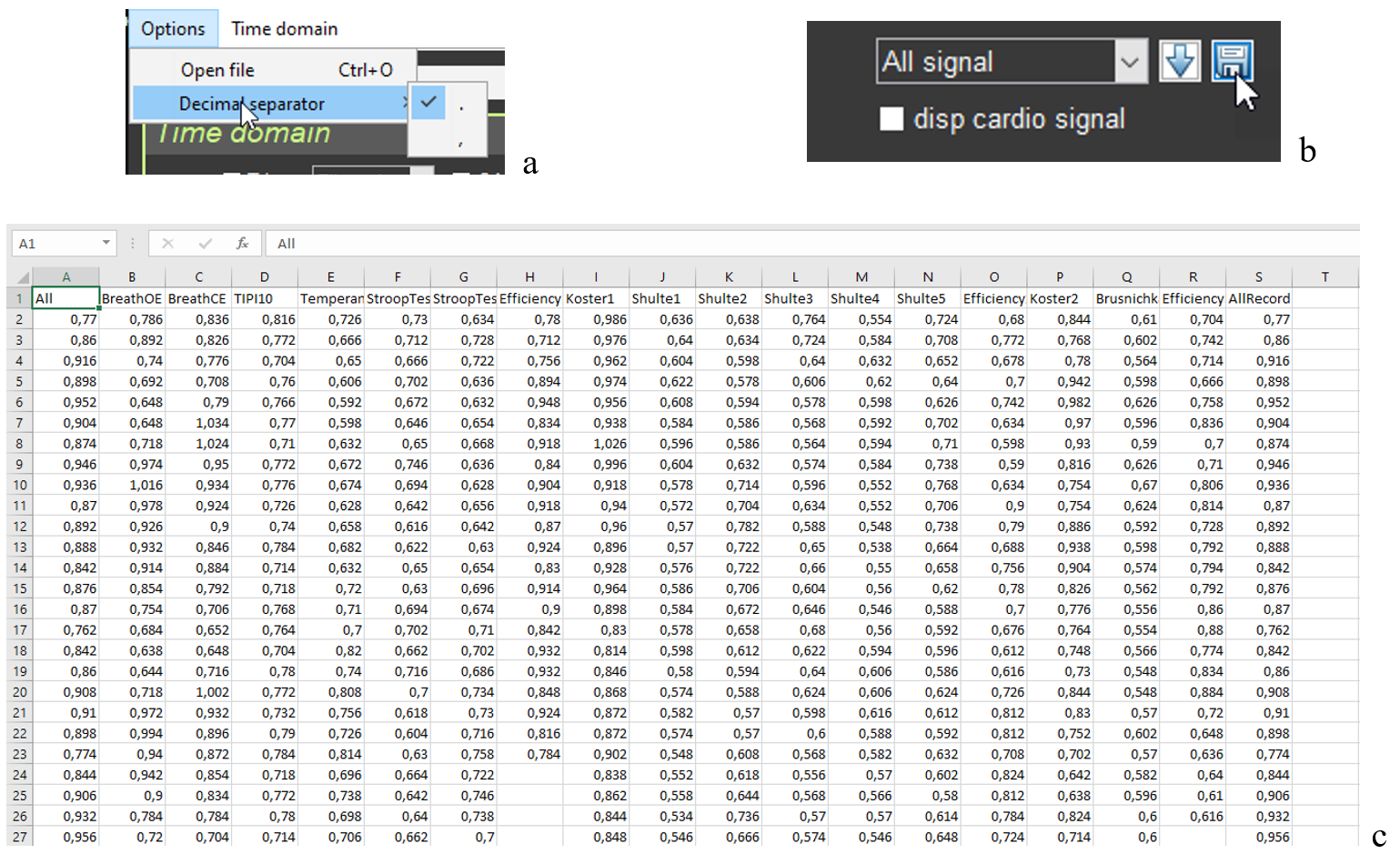
The ability to work with digitized raw data is important primarily for scientific work, which in the future involves using programs with statistical processing capabilities. And here it is important to know which symbol after the integer value is used to separate fractional values. This is because some statistical programs “work” with a dot, some with a comma. Therefore, before becoming acquainted with the possibility of saving RR interval data, let us turn to the “Option” window on the top panel (Fig. 1.2a). Only now do we activate the “Decimal separator” line (Fig. 2.3a). It is clear that this window allows you to choose the symbol with which the digitized raw data will be saved.
Choose the one you need and click on it.

Next, we turn to sector 1 to the “button” with the floppy disk image – a classic sign of saving something (Fig. 2.3b). This action will prompt you to save RR interval data in a file with the “csv” extension to the same folder that was created in “SAVED DATA” for a particular person.

The file with the saved RR interval data, expressed in seconds, opens in Excel (Fig. 2.3c). RR intervals are sequentially located in named columns: for the entire study period (All) and for each stage separately.

Figure 2.3. Sequence of actions for saving RR interval data (explanations in the text)

Sector. 1.4

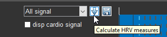
It is impossible to describe the button with the arrow pointing downward (Fig. 2.4) without references to other sectors and work with functional buttons.
Let us sort it out.

Figure 2.4. Button that allows you to recalculate HRV data for the ECG segment selected by you in the sector.

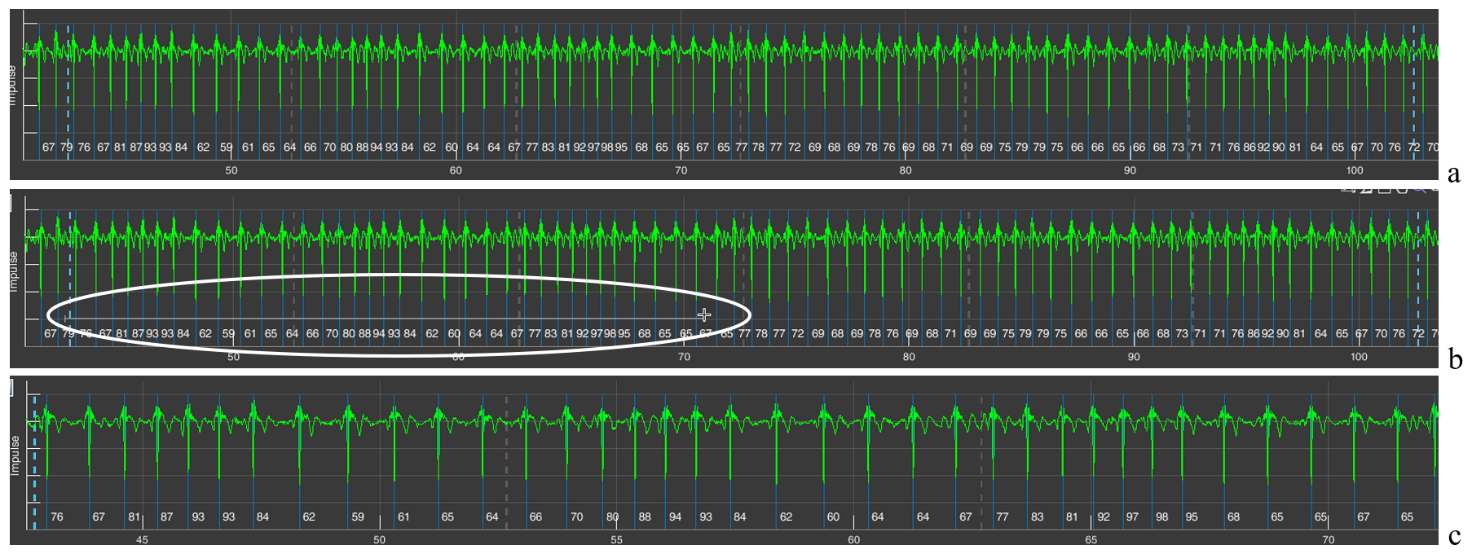
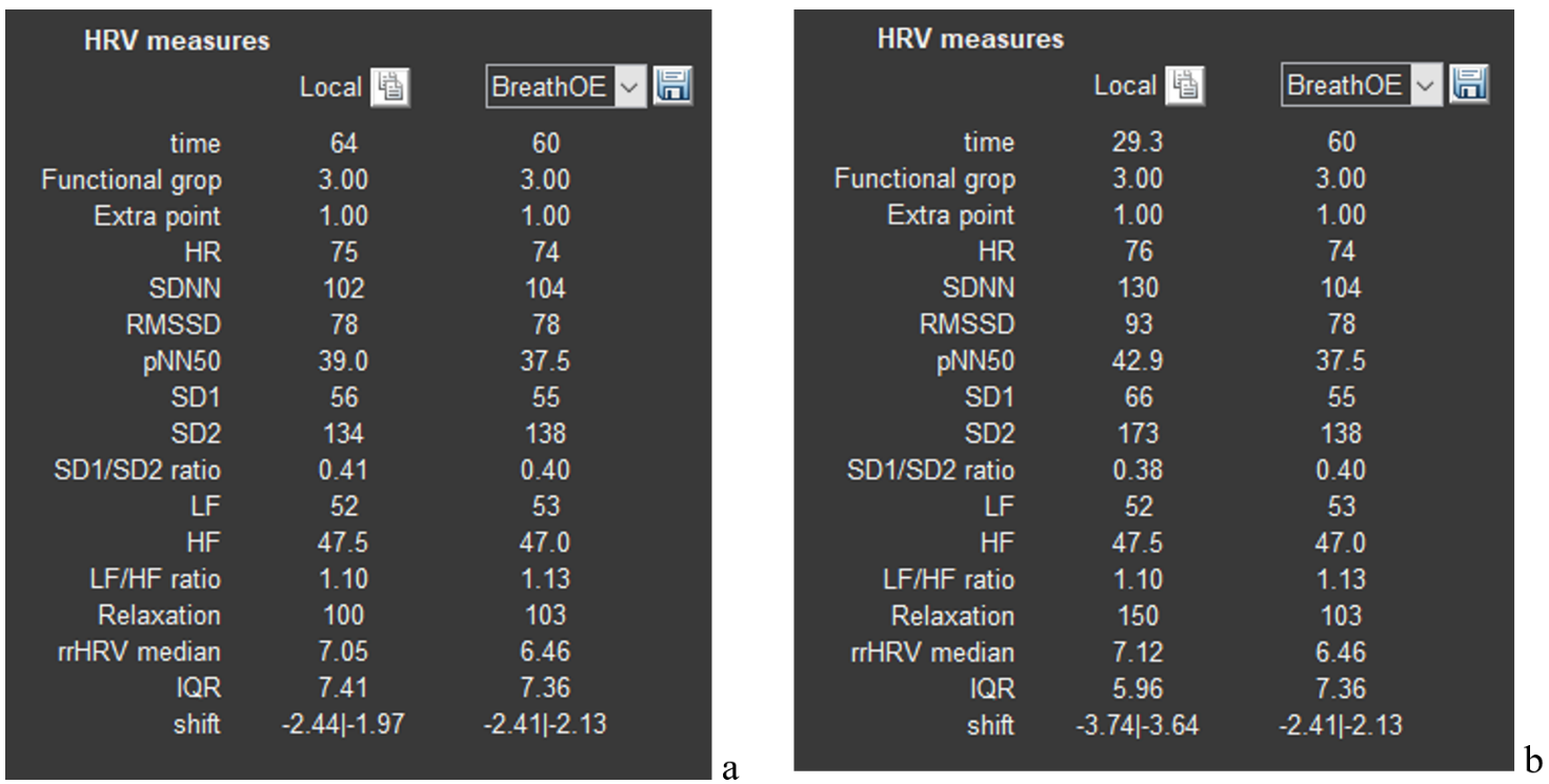
For this we will have to refer to sector 4 and the ECG segment already displayed by us, which corresponds to the BreathOE stage (Fig. 2.5a). We immediately draw your attention that the duration of the BreathOE stage is visualized in the sector window from one vertical dashed blue line to another, but the window includes a somewhat larger segment. It is precisely the HRV data for the entire window that are displayed in sector 3 under the “Local” label, and under the window in which the BreathOE stage is displayed – data only for the time of the stage itself (from one vertical dashed blue line to another). This nuance becomes clear if we refer to the first line “time”: under the “Local” label – 64 seconds; under “BreathOE” – 60 (see Fig. 2.6a).

If you want to know, for example, what the HRV measures were in the first half of the stage, then you must display this time interval in the sector 4 window. We recall the “+” icon in the upper right corner. Move the cursor to this area of the sector 4 window, functional buttons will be activated, press “+” and bring the cursor to the beginning of the stage (the first vertical dashed blue line) already in the form of a small cross, hold down the left mouse button and draw a horizontal line to the place we need (Fig. 2.5b; according to our example, this is the middle of the BreathOE stage; our actions are highlighted with a white oval) and release the mouse button. The result of these manipulations will be reflected in the sector 4 window, namely, displaying the selected time interval of the ECG on it (Fig. 2.5c).

Figure 2.5. Sequence of actions for changing the scale of the ECG curve (explanations in the text)

Let us check. We look at the lowest line that reflects the time of the study (Fig. 2.5a). As we can see, the BreathOE stage lasted between the 40th and the 110th seconds. The time we selected is already between the 40th and the 75th seconds (Fig. 2.5c). We did everything correctly.

Now you can press the arrow button as well. We press it and look at sector 3. If at first, under the “Local” label, HRV data were displayed for the period of 64 sec., which included the BreathOE stage, and under the window in which the BreathOE stage is displayed – data only for the time of the stage itself (Fig. 2.6a), then after pressing the arrow button, under the “Local” label, HRV data appeared for the period that we displayed on the sector 4 screen, and under the window in which the BreathOE stage is displayed, HRV data only for the period of the stage itself were preserved (Fig. 2.6b).

Figure 2.6. a – HRV data after visualizing the BreathOE stage in sector 1; b – HRV data after the time interval of the ECG curve we selected in sector 4.

Changes will also occur in sectors 5, 6, and 8. Which ones? This was described above and shown in Figure 2.3.

We hope that we have sorted out sector 1. We will move on.

Sector. 2

Sector 2 reflects the respondent’s anthropometric data.

This sector does not require special explanations, except for one point (Fig. 2.7).

Figure 2.7. A sector on the screen with the respondent’s anthropometric data (explanations in the text).

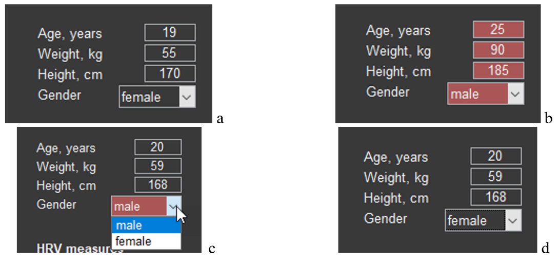
Data on the number of full years, weight, height, and sex can be displayed in the main tone of the screen (Fig. 2.7a) or in red (Fig. 2.7b). Red is always a warning color: these data do not correspond to the respondent. Such cases can occur, for example, when you changed the names of the main files, accidentally deleted the file for storing these data in the “SAVED DATA” directory (remember our warnings?) or activated with CleverView a file from another location. The possibility of correctly assessing results related to HRV is possible only with reference to the data of sector 3. Therefore, if you need data for a particular person and the cells of the sector are colored red, enter them manually (age, weight and height) and, using the arrow (Fig. 2.7c), specify sex. The result obtained is shown in Figure 2.7d.

It remains to do a recalculation. Press the arrow of sector 1 (Fig. 2.4). Now the HRV data from sector 3 can be saved for further work with them.

Sector. 3

Sector 3 is a table with HRV data for the study period activated in sector 4, and selectively by stages for comparison. This sector also includes the ability to save HRV data as a separate file in Excel.

We have already become acquainted with the table itself (see Fig. 2.6). Now let us consider it in more detail. Something will have to be repeated, something reminded.

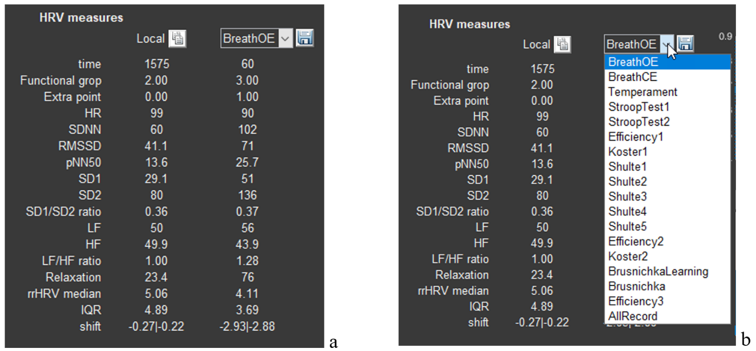
The table itself is labeled “HRV measure” (HRV – Heart Rate Variability) and consists of 3 columns: the 1st contains a list of HRV measures; the 2^nd – “Locale” – contains the measures corresponding to the first column for the study period that is displayed in sector 4 (when we load the required file, sector 4 displays the ECG for the entire study period (Fig. 2.8a). If in sector 1 we select one of the stages, then in this column the HRV data of the stage we selected, displayed in sector 4, will be shown (Fig. 2.6a)); the 3rd, as its title, contains a window with an arrow, clicking on which opens another window with a list of the stages of the study passed by the respondent (Fig. 2.8b). Earlier we selected the “BreathOE” stage (Fig. 2.6b).

Figure 2.8. a – HRV data after activating the respondent’s file; b – selection of a stage for displaying HRV data in the second column of the table.

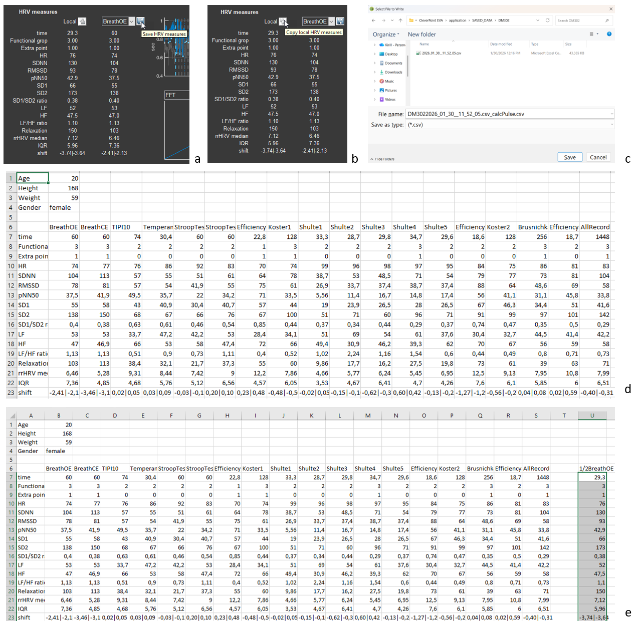
Now let us save the HRV data (Fig. 2.9). Move the cursor to the “button” with the floppy disk icon (Fig. 2.9a). Click, and you are prompted to save the data in the person’s folder in the “SAVED DATA” directory in a file whose name is the name of the main file with “_calcPulse” added (Fig. 2.9c). The saved file can be opened in Excel; the main sheet is illustrated in Fig. 2.9d.

Figure 2.9. Saving HRV data (explanations in the text)

If you remember, when we analyzed sector 1, we were “interested” in what the respondent’s HRV response was at the beginning of the test with slow controlled breathing with open eyes (Figs. 2.5 and 2.6b). The data in the “Local” column are non-standard and are not included in the saved file with HRV data (Fig. 2.9d). However, if they are of interest to you and are needed for any purposes, you can save them by pressing the functional button (standard for such purposes) next to the text “Local” (Fig. 2.9b). The data of this column will be loaded into the clipboard, and you can save them, for example, in the file created by CleverView in a separate column. In our example, we called it “1/2BreathOE” (Fig. 2.9e).

Separately, as briefly as possible, we will dwell on heart rate variability measures (Table 1).

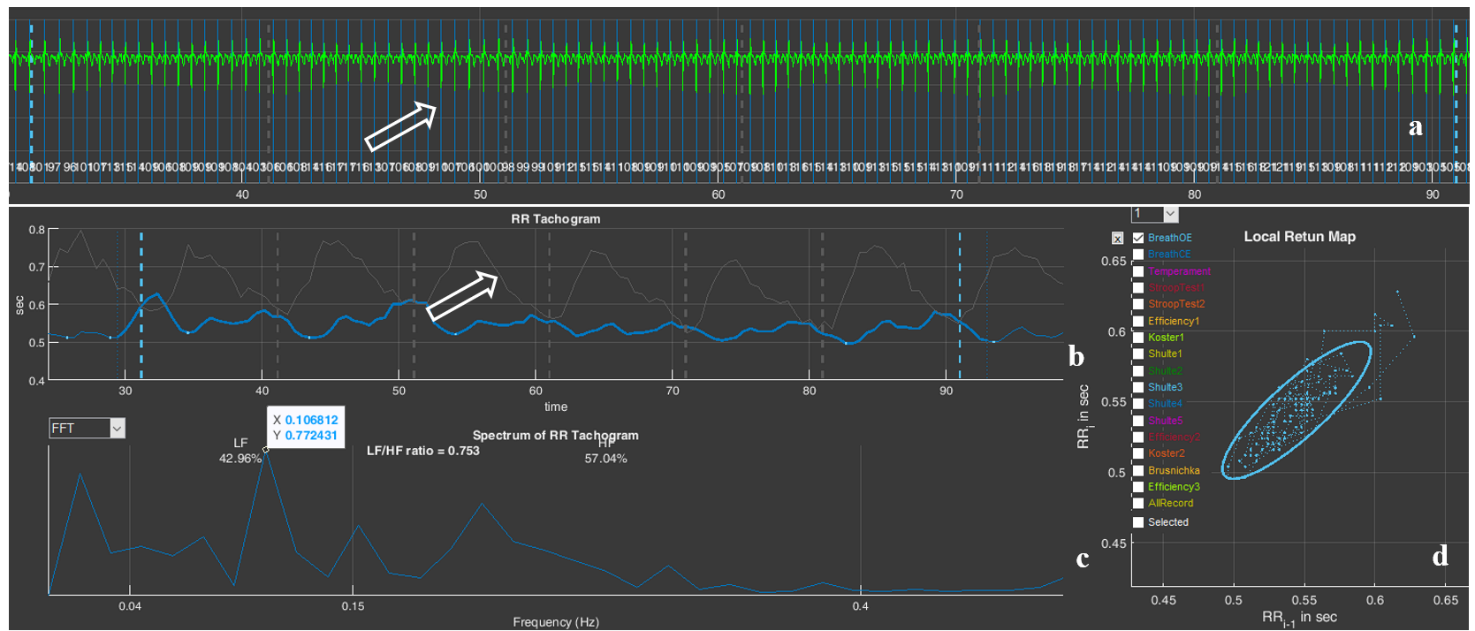
The duration from one heart contraction to the next is not the same. This is clearly seen in the ECG example we recorded in sector 4, and visually, but more convincingly, this is confirmed by the numbers next to each vertical blue line (Fig. 2.10). These numbers reflect the value of the instantaneous heart rate (HR), which is calculated over the length of one interval between R waves of successive ECG complexes: 88, 94, 93, 84, 62, 60 beats/min (the classic labeling of the ECG complex waves is shown on the fourth ECG complex window from the beginning). This non-uniformity of the duration between heart contractions is called heart rate variability (HRV).

Figure 2.10. Example of heart rate variability

Reminder: (1) In our ECG graphs, the ECG is presented in an inverted form; (2) The main purpose of displaying the ECG in Sector 4 is to enable visualization of the correctness of the automatic detection of the R wave, which is marked by a vertical blue line.

HRV analysis in CleverView is based on measuring intervals between R waves on the ECG and constructing a cardiointervalogram – a graphical representation of the durations of successive RR intervals (see the graph in sector 5, where the horizontal axis shows the time of the ECG recording, and the vertical axis shows the duration of the RR interval). Then the RR-interval data are processed using various mathematical methods. What does heart rate variability depend on? First of all, on the tone of the systems responsible for regulating the pumping function of the heart, and above all on the functional state of the autonomic nervous system. The autonomic nervous system consists of two subsystems that perform different functions in the body: the sympathetic nervous system and the parasympathetic nervous system. In the most simplified terms: the sympathetic nervous system maintains the functioning of the body in a stressful situation, and the parasympathetic system supports recovery processes after stress.

There are many mathematical approaches to processing RR intervals and assessing HRV. Measures from some of them are used in CleverView. These are the ones displayed in the table of sector 3. You can see the interpretation of these measures in Table 1.

Table 1. Sector 3 measures, their definition and physiological role.

We caution you against a mechanical interpretation of HRV data and categorical conclusions! HRV is a vast body of scientific views, approaches, and conclusions. The results and their interpretation depend on many nuances, some of which have been taken into account by the CleverView developers, but many still require scientific consideration. The researcher’s personal experience is also important—their accumulated data and the set of individuals associated with them, with whom they have worked.

Let us move on.

Sector 4

Sector 4 displays a graph of automatically detected R waves on the ECG, and when the corresponding cell in sector 1 is activated (see Fig. 2.2a) it also displays the ECG curve itself. We have already become familiar with this part (see the subsections: “Sector 1.1”, “Sector 1.2”, “Sector 1.4”). By and large, the function of this sector is described and understood. It remains, using the example of some ECGs in sector 4, to consider working with the functional icons that we briefly described in Chapter 1.

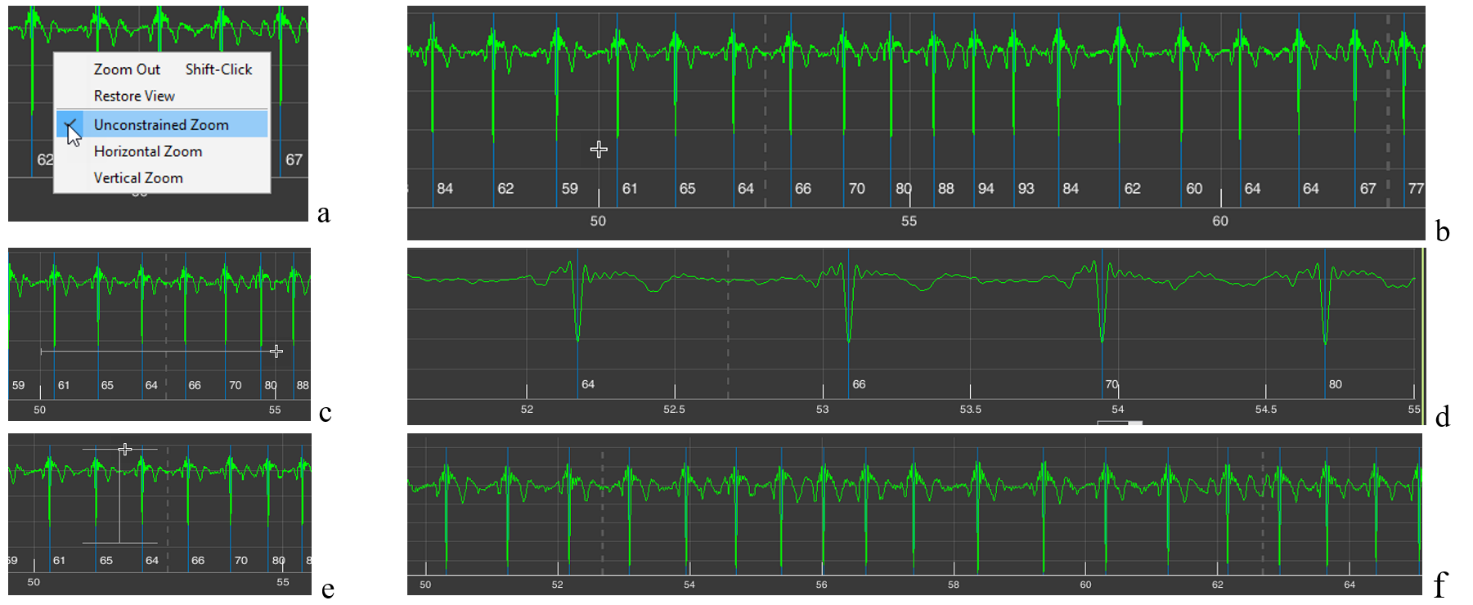
Let us begin with the already familiar “+” icon – “Zoom In” (Fig. 1.8f). If, after activating this icon (the active icon is colored blue), you move the cursor over the image in sector 4 and press the right mouse button, a window with a list of further actions will appear (Fig. 2.11a). By default (the selected line is additionally highlighted when the cursor is placed on it), the function is active that allows you to enlarge the image both horizontally (we considered horizontal enlargement when describing the subsection “Sector 1.4”) and vertically. The choice of direction is up to you. If, by pressing and holding the left mouse button, you select a horizontal segment, the ECG will be stretched horizontally, i.e., along the time scale (Fig. 2.11c, d); if you select a segment of the ECG vertically, the ECG will be enlarged on the screen by amplitude within the selected range in the sector window (Fig. 2.11e, f).

Figure 2.11. Possibilities for changing image scaling in sector 4 when the “+” icon is activated by default or when the “Unconstrained Zoom” line is activated (explanations in the text)

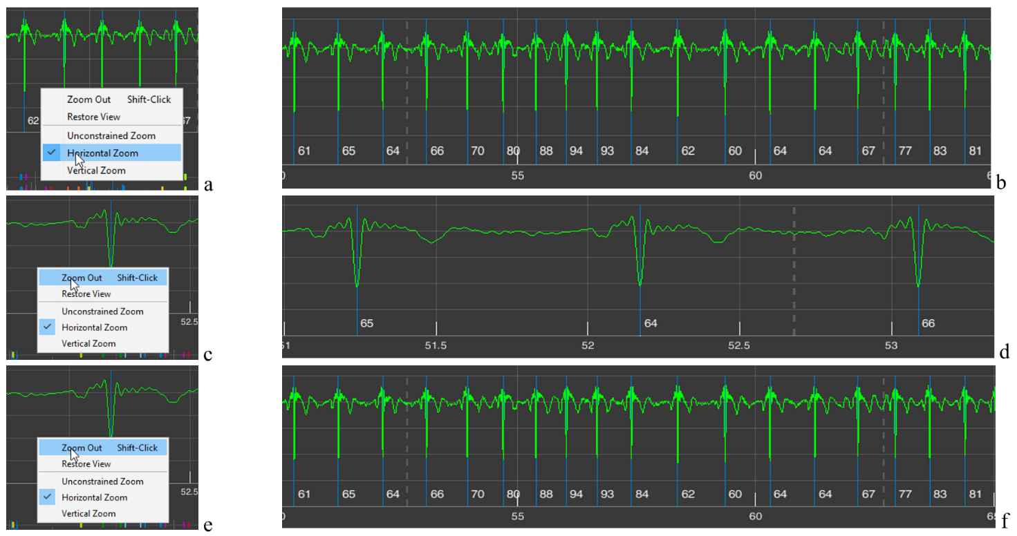
Sometimes such a function is inconvenient for someone. Then, by activating the “Horizontal Zoom” (Fig. 2.12a) and/or “Vertical Zoom” (Fig. 2.12c) lines, you can choose the required direction for scaling; in this case, the cursor will not be in the form of a cross (Fig. 2.11b) but with arrows indicating the selected direction (Fig. 2.11b and d).

Figure 2.12. Possibilities for changing image scaling in sector 4 when the “Horizontal Zoom” and “Vertical Zoom” lines are activated (explanations in the text)

The “Zoom Out” line is activated when you click on it (Fig. 2.13c). In this case, the scaling process you performed earlier is cancelled step by step (Fig. 2.13a – stretching the time scale; see Fig. 2.13 from b to d) (Fig. 2.13e, f).

Figure 2.13. Changes in image scaling in sector 4 when the “Zoom Out” line is activated (explanations in the text)

The need to repeatedly activate the “Zoom Out” line is not always convenient. Therefore, you can click (activate) the “Restore View” line (Fig. 2.14a) and return to the image in sector 4 that appears upon loading (Fig. 2.14b), and then, by activating the “+” icon, return to the required time point and the desired zoom level.

Figure 2.14. Changes in the image zoom in sector 4 when the “Restore View” line is activated (see explanation in the text)

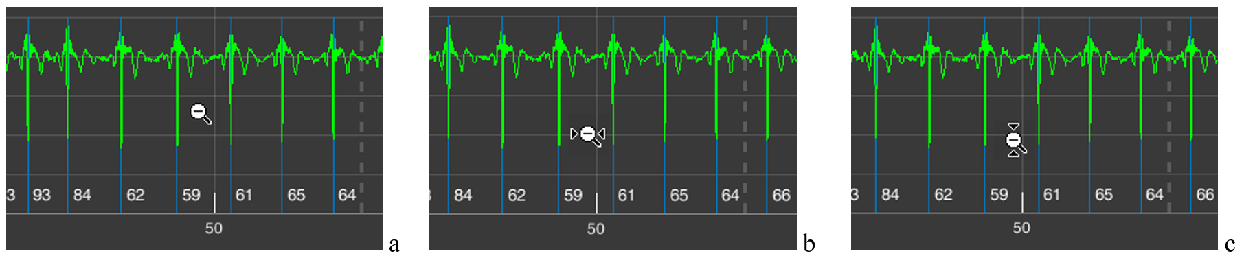
The same result, of returning back to a more compressed time scale or ECG-signal amplitude, can be achieved if you activate the “-” icon – “Zoom Out” (Fig. 1.8g). In this case, the additional window that appears (Fig. 2.11a) will be the same. But the cursors will have the “-” sign (Fig. 2.15). A click with the cursor without arrows (Fig. 2.15a) will reduce both the vertical and horizontal scale step by step; with horizontal arrows (Fig. 2.15b) – the time scale; with vertical arrows (Fig. 2.15c) – the amplitude scale.

Figure 2.15. Cursors with the “-” icon active: a – when the “Unconstrained Zoom” line is activated; b – the “Horizontal Zoom” line; c – the “Vertical Zoom” line

The same result as with the “Restore View” line can be obtained by activating the icon with a house, which is also called “Restore View” (Fig. 1.8g). Therefore, in the future we will not return to this icon.

As we can see, the same result can be achieved in different ways. Which is better? This is at the discretion of the researcher: to choose the way of working with the CleverView page that is convenient or familiar to them.

Icon with the image of a paint brush – “Brush/Select Data” (Fig. 1.8c). Activate it and, while holding down the left mouse button, select the area that you want to highlight in a different color (Fig. 2.16a), and release the mouse button. The result is shown in Fig. 2.16b. To remove the color highlighting, it is enough to click once while keeping the cursor in the area of the background (black) field.

Figure 2.16. Result of actions when the “Brush/Select Data” icon is active (explanations in the text)

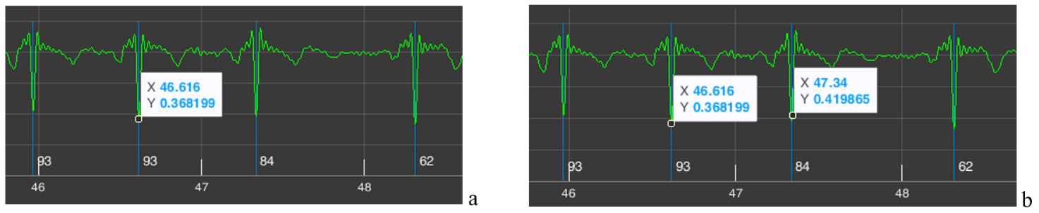
Icon depicting lines in a window – “Data Tips” (Fig. 1.8d). We remind you that with its help you can determine the coordinates of a point on the curve that interests us. To do this, activate the icon, move the cursor to the required place on the curve, click the left mouse button, and obtain a coordinate window (Fig. 2.17a). If necessary, the position can be adjusted with the “<” and “>” arrows on the keyboard. The “X” axis shows time, the “Y” axis shows signal amplitude (for the ECG on our scale, in V (volts)). By holding down the “Alt” key, you can place data for a larger number of points on the curve (Fig. 1.17b).

Figure 2.17. Result of actions when the “Data Tips” icon is active (explanations in the text)

In our example, we marked on the ECG two consecutive R waves. Let us recall that next to the blue line marking the R wave, the value of the instantaneous HR is indicated below – 84 for the second “our” R wave. Let us check. The time of appearance of our first R wave is 46,616 seconds, of the second – 47,340 seconds. We calculate the duration of the RR interval: 47,340 s – 46,616 s = 0,718 s. Now let us calculate what the HR would be with such an interval between successive heart contractions: HR = 60/0,718 = 83,6 beats/min, or ≈ 84 beats/min. We conclude that the automatic calculation is correct.

The next functional icon is “Pan” (Fig. 1.8e). Activating the hand-shaped icon causes a similar cursor to appear on the screen. Working with it is very simple: place the cursor on our ECG curve, hold down the left mouse button, and slightly move the mouse in different directions. Everything is very clear and, we hope, does not require special explanations of what this function is needed for.

And we need to move on.

Sector 5

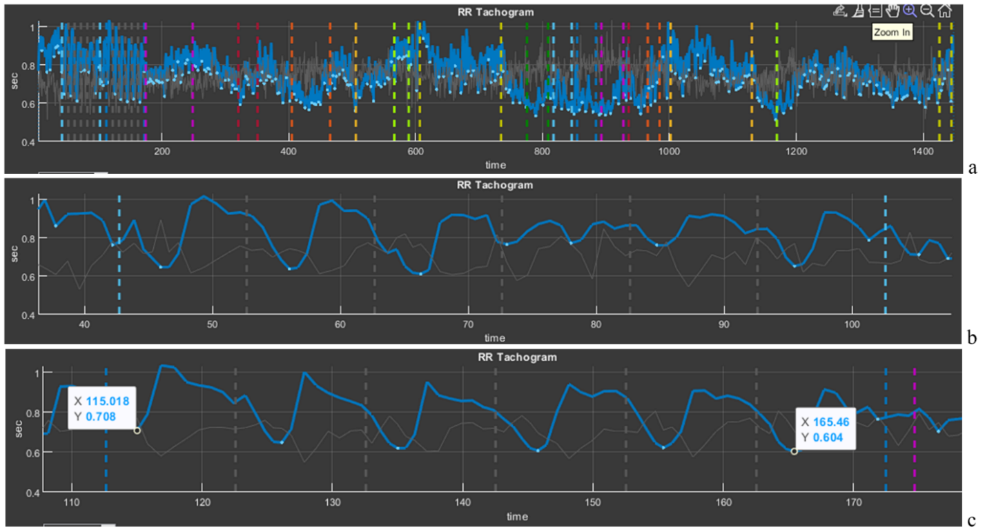
Sector 5 displays a cardiointervalogram (CIG), which reflects the dynamics of RR intervals (Fig. 2.18b). We already mentioned the CIG when we talked about HRV. This curve is a visual illustration of HRV as a whole. Let us consider it in more detail.

Figure 2.18. Cardiointervalogram for the entire study period

On the horizontal axis (“time”), the study time is plotted; on the vertical axis, the value of the RR interval (in our figure from 1 s to 0,4 s). We draw your attention to the fact that the shorter the RR interval, the higher the HR, and vice versa (1 s corresponds to 60 beats/min, 0,4 s – 150 beats/min). Therefore, you need to get used to this curve in order to interpret it correctly: if the CIG curve crawls upward, it means that the heart began to beat less frequently; downward – faster. A few more points for evaluating the curve of sector 5: a wide curve – high HRV, a narrow one – low; a flat curve – an inert regulatory system that ensures the work of the heart; pronounced fluctuations in the level of RR intervals (as in Fig. 2.18) – a mobile one.

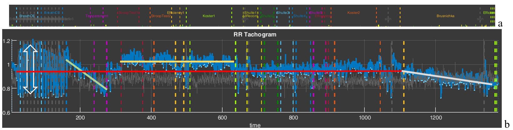
We also remind you of the color marking of the study stages. For a better idea of where which stages are, we supplemented Fig. 2.18 with Fig. 1.5 from the “Time domain” page (Fig. 2.8a). Let us draw your attention to the stages with slow breathing (6 breathing movements per minute), the stage for the speed of pressing the controller key (“Temperament”), the stages with cognitive load (“Stroop” 1,2, “Shulte” 1-5 and “Brusnichka”), and the stages where the respondent was offered to rest (“Koster” 1 and 2). We will return to Fig. 2.18b in the next chapter; for now we only note how the duration of RR intervals changes, and, consequently, HR.

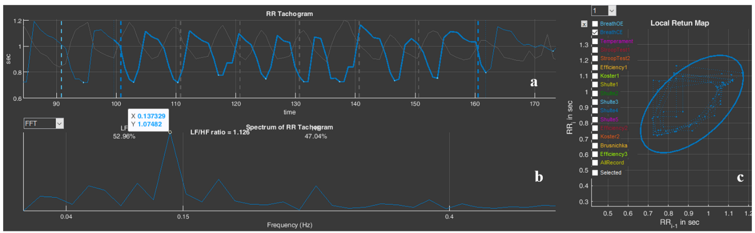
And let us also consolidate, using the example of this sector, the work with the functional icons. Move the cursor to the upper right corner and select “Zoom In” (Fig. 2.19a). Now, along the horizontal axis, select the stage of slow breathing with open eyes “BreathOE”, marked with light-blue dashed vertical lines. As a result, only this stage is selected on our screen in sector 5 (Fig. 2.19b). It can be seen how HRV has “swung” against the background of such breathing, especially at its beginning (the dependence of HRV on breathing is a normal phenomenon and is called respiratory arrhythmia). Now press “Restore View”, the CIG returns to its original form, and now select the stage of slow breathing with closed eyes “BreathCE” (Fig. 2.19c). If we compare the stages of slow breathing with open and closed eyes, it is noticeable that during closed eyes HRV is more stable and throughout coincides with the phases of breathing. However, if we mark reference points on the curve (in our case we chose the lowest values of the respiratory arrhythmia wave) at the beginning of the test and at the end using the “Data Tips” icon, we will see that the RR interval decreases from 0,708 s (or ≈85 beats/min) to 0,604 s (or ≈99 beats/min) (Fig. 2.9c), i.e., the already increased heartbeat begins to beat even more often. It can be assumed (we emphasize, “assumed”) that the test with controlled slow breathing is performed by the respondent with strain; however, the heart-rate regulation system responds to slow breathing with a frequency of 6 breathing movements per minute: between the vertical dashed blue lines (the duration of the “BreathCE” stage is 1 minute) 6 waves of oscillations in the duration of RR intervals are visible, which indicates a relatively synchronous “work” of the external respiration systems and the control of heart contractions (Fig. 2.19c).

Figure 2.19. Selection of cardiointervalograms at slow breathing stages (explanations in the text)
Above we provided a modest example of the possibility of interpreting data of a person’s physiological response to tasks in VR (in our examples, this is a response to tests in Stressonika), which can be done using CleverView. We will “work” with examples in more detail and in greater depth in the next chapter.

Sector 6

Sector 6 by default displays a spectrogram of the dynamics of RR intervals for the entire study period (Fig. 2.20). A spectrogram is a graphical representation of the performed spectral analysis of a sequence of RR intervals. If you look at the CIG (Fig. 2.18), you can see that the RR-interval values fluctuate, and the CIG itself consists of both fast and slow oscillations. Spectral analysis makes it possible to identify which frequencies make the greatest contribution to the pattern of the cardiointervalogram. All possible frequencies (see the horizontal scale in Fig. 2.20) fit in the range from 0 to 0,5 Hertz (Hz). Classically, the following are distinguished: the very low frequency range, or VLF (up to 0,04 Hz), the low frequency range, or LF (from 0,04 Hz to 0,15 Hz), and the high frequency range, or HF (above 0,15 Hz). Spectral analysis is most informative when the duration of the ECG recording in a certain stationary state is 5 minutes or more.

Under the conditions of testing in Stressonika, the recordings are short. Therefore, only the low-frequency (LF) and high-frequency (HF) ranges and their ratio are digitized in sector 6 (Fig. 2.20).

Figure 2.21. Spectrogram of the dynamics of RR intervals for the “BreathOE” stage

We remind you that work with sector 6 is related to work in sector 1; for example, activating the “BreathOE” stage in sector 1 will lead to recalculation of the spectrogram only for this stage (Fig. 2.3). Let us consider the resulting spectrogram more closely (Fig. 2.21).

Figure 2.21. Spectrogram of the dynamics of RR intervals for the “BreathOE” stage

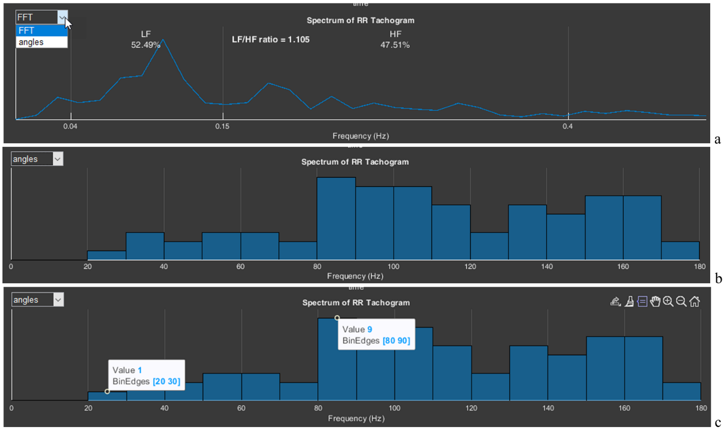
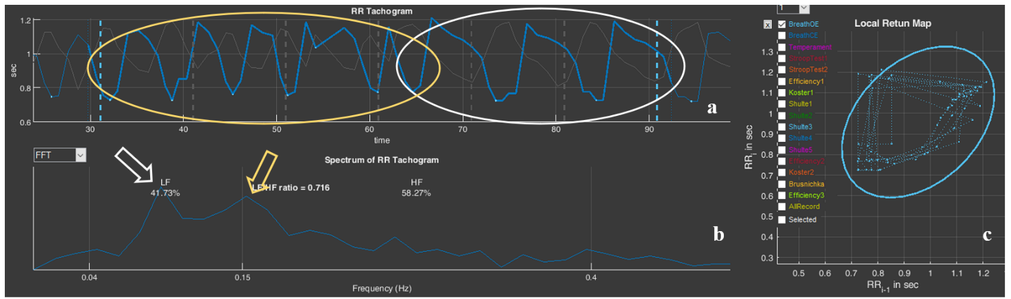
We draw attention to the fact that the spectrogram shows a slight dominance of the low-frequency range (52,49%), which was also reflected in the LF/HF ratio (it is greater than 1). Using “Data Tips”, let us mark the peak on the spectrogram: frequency – 0,107 Hz (or 6,4 per min); amplitude – 0,862 ms2. And now let us look at Fig. 2.19a. This is what the sequence of RR intervals looks like, on the basis of which this spectrogram was built. As we remember, this is related to the task of slow (6 breathing movements per minute), rhythmic, imposed breathing with open eyes. Ideal performance of this test would appear in the form of a high-amplitude sinusoid-like CIG curve with 6 waves. The CIG graph presented in Fig. 2.19a resembles such a curve only very remotely, which is confirmed by spectral analysis: a moderate predominance of LF, the frequency characteristic of the peak on the spectrogram differs somewhat from the frequency of the imposed rhythm (0,1 Hz), and the peak amplitude is less than 1.

This example is also only for becoming acquainted with the “Cardio domain” page. We will consider details and specifics in the next chapter.

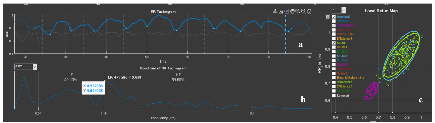
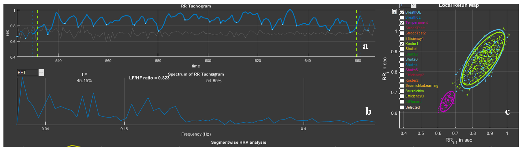
In the upper left corner of sector 6 there is a window that allows the spectrogram to be replaced with an angle histogram on the scatter plot located in sector 7. To do this, it is necessary to activate the list for selecting the image in sector 6: FFT (Fast Fourier transform) – to select the spectrogram; “angles” – to select the angle histogram (Fig. 2.22a). By default, a spectrogram is displayed in the sector; if we select “angles”, an histogram is displayed (Fig. 2.22b). The step of our histogram is 10°, and the height of a bar is the number of angles that were recorded in this range (Fig. 2.22c: range 20-30° – 1 angle, 80-90° – 9). The histogram clearly shows which angles were more frequent at the stage activated in sector 1 (Fig. 2.3b). In Fig. 2.22b it is clearly visible that during the “BreathOE” stage there were more angles exceeding 90°. It is considered that when the sympathetic nervous system is activated, the histogram density shifts to the left, i.e., toward acute angles.

Figure 2.22. Stages of switching from a spectrogram to an angle histogram on the scatter plot (explanations in the text).

This HRV assessment approach is one of the geometric methods.

Sector 7

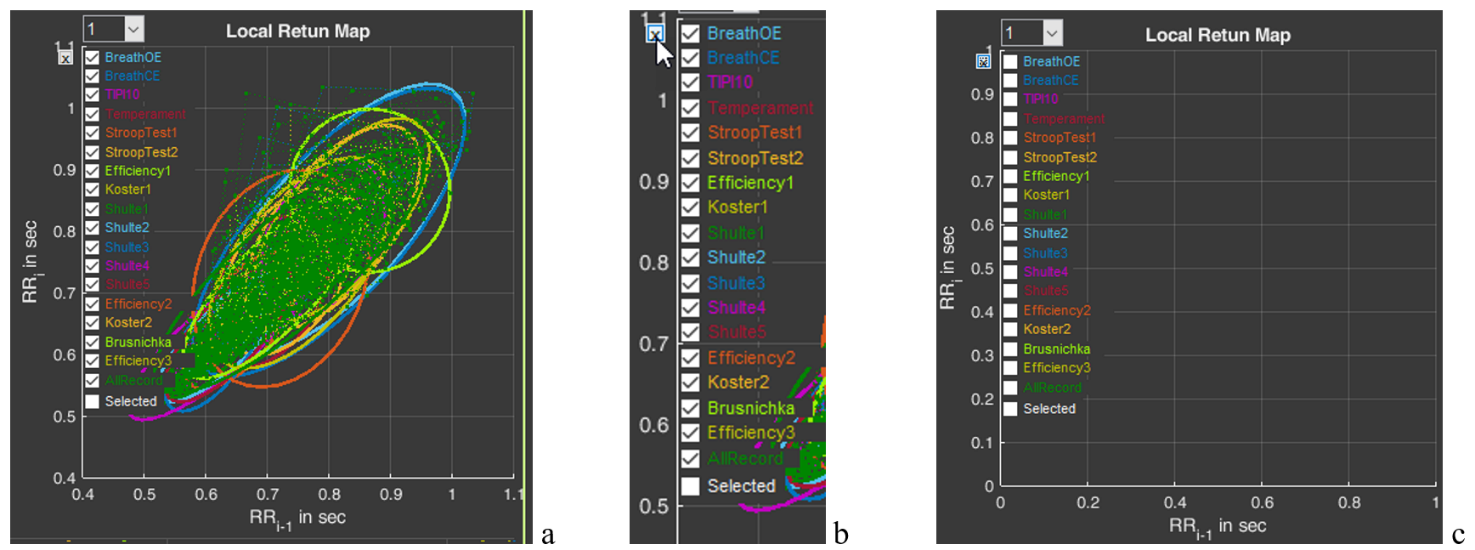
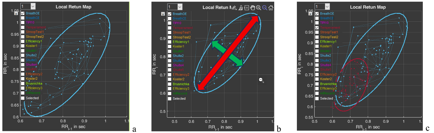
Sector 7 contains a scatter plot, or a Poincare plot. With respect to HRV, this is a graphical method for displaying the relationship between successive R-R intervals (cardiac cycles). When constructing this plot, the position of each point is determined by two coordinates: on the ordinate axis (vertical axis) – the duration of the RRi interval, on the abscissa axis (horizontal axis) – the preceding one, RRi-1 (Fig. 2.23a). By default, the sector immediately displays plots for all stages (Fig. 2.23a). On the left side, a column is displayed with the names of all these stages (in our example, Stressonika), marked with the corresponding color (as are the plots in the sector) and with a window where the activation mark is set (Fig. 2.23b). You can visualize the stages that interest you by removing the activation mark or setting it. You can clear the plot field at once by clicking on the cross in the upper left corner (Fig. 2.23b). The result of this action is shown in Fig. 2.23c.

Figure 2.23. HRV Poincare plot in sector 7 and the ability to control the image on the plot (explanations in the text)

Activate the Poincare plot on the graph only for the “BreathOE” stage (Fig. 2.24a). We remember that the plot scale can be controlled using the functional icons (Fig. 2.24b). It is possible to activate plots not for one, but for several stages for comparison (Fig. 2.24c).

Figure 2.24. HRV Poincare plot for the “BreathOE” stage (explanations in the text)

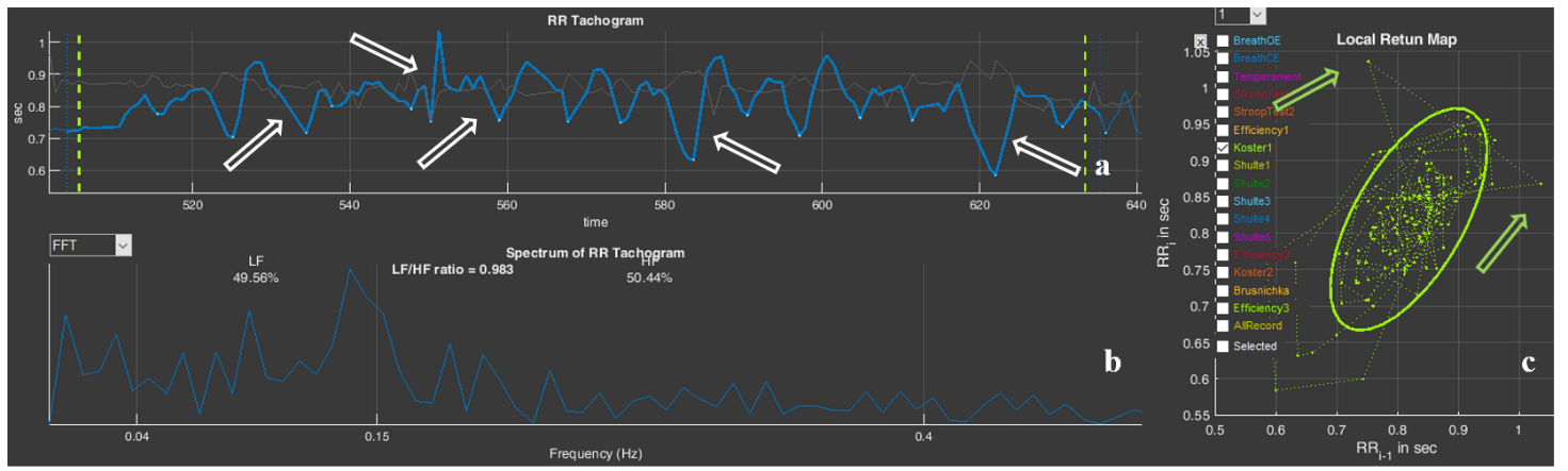
Now a few words about the scatter plot. The HRV Poincare plot is a visual representation of the integral picture of HRV, which makes it possible to assess the activity of regulatory systems by the shape of the “cloud” of points: a compressed cloud may indicate low variability; by the location of the cloud one can judge HR (we remind you that the smaller the RR-interval value, the higher the HR, and vice versa); the symmetrical shape of the oval outlining the cloud and its optimal form indicate a balance of the autonomic nervous system; significant outliers of points beyond the main cloud most often indicate a significant rhythm disturbance.

The cloud itself is assessed by the shape of the oval drawn around it and by the values of SD1 (the width of the cloud – the green arrow), SD2 (the length of the cloud – the red arrow) (Fig. 2.24b) and their ratio SD1/SD2 (see Table 1).

Using the plot, it is possible to: trace how the body adapts to stress (in the case of Stressonika, this is cognitive stress); assess the balance between the sympathetic and parasympathetic divisions of the autonomic nervous system; track how HRV changes over time under the influence of certain effects, for example, breathing practices.

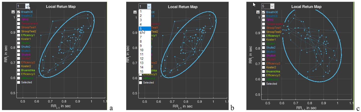
And one more function of sector 7 is the window with the number 1 (Fig. 2.254a). The number can be changed by activating this window (Fig. 2.25b). For example, we selected the number 5 (Fig. 2.25c). As can be seen, the shape and position of the cloud have changed. This is because on the abscissa axis we selected not the value RRi-1, but the value RRi-5. This function is needed to search for an autocorrelation dependence. But this is already for very advanced scientific research work.

Figure 2.25. Search for an autocorrelation dependence using the “BreathOE” stage as an example (explanations in the text)

Sector 8

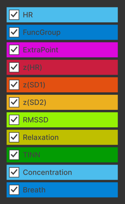
In sector 8, by default, graphs are combined that reflect the dynamics of a fairly large number of calculated indicators of a person’s functional state (Fig. 2.26).

Figure 2.26. Graphs of sector 8

Definitions of the sector graphs and their color marking are presented in Table 2.

Most of the indicators have already been described above. “New” for you may be the indicators z(HR), z(SD1), z(SD2) and TINN. The z index for the HR, SD1 and SD2 indicators shows how the respondent’s result relates to the values of the same indicator among all persons of the same age and sex. The definition of the TINN indicator, or triangular index, is complex: the integral of the distribution density divided by the maximum of the distribution density. It is clear that monitoring it is intended for scientific activity.

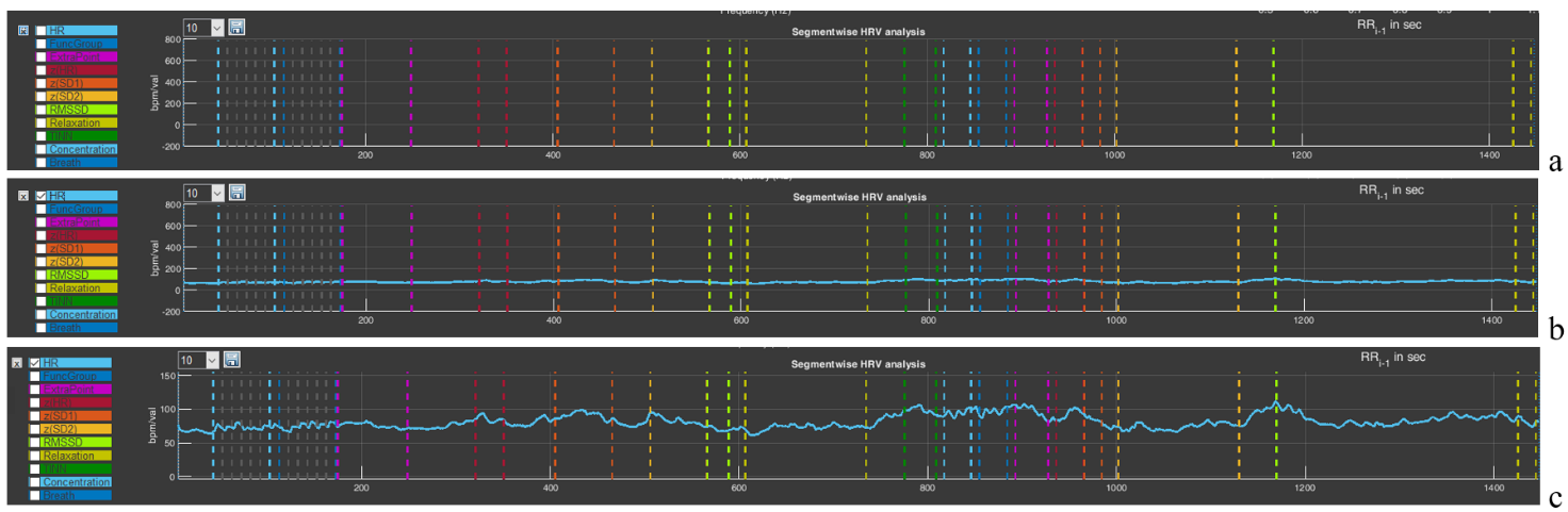
Now let us consolidate the already familiar skills of using the functional capabilities for controlling the image. Click on the cross in the upper left corner of the panel with the list of graphs in sector 8 (see the figure in Table 2). As we remember, it clears all images on the plot (Fig. 2.27a). Activate the graph of the indicator that interests us, for example, HR (Fig. 2.27b). Using the “+” icon (“Zoom In”), scale the graph along the vertical axis so that the dynamics of the indicator are visible (Fig. 2.27c).

Figure 2.27. Selecting a graph in sector 8 (explanations in the text)

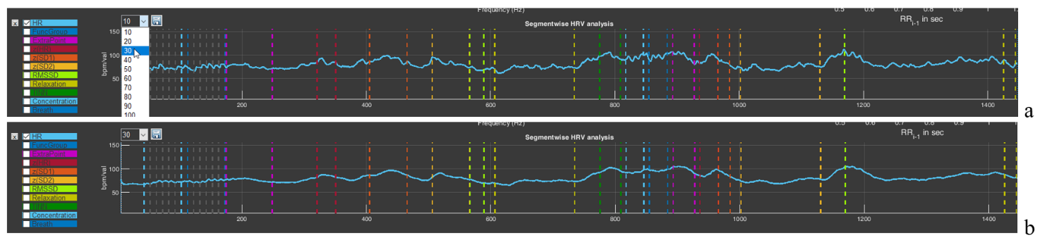
The window with the number 10 will allow you to build a graph with averaging of the number of points specified in the window. By default, a graph is built with averaging of 10 points. But you can select a larger number of points for averaging (Fig. 2.28a). This will lead to “smoothing” of the graph (Fig. 2.28b), which is sometimes useful if the spread of instantaneous values is large, which makes it difficult to see the general trend of changes in the indicator during a VR session.

Figure 2.28. Graph smoothing function in sector 8 (explanations in the text)

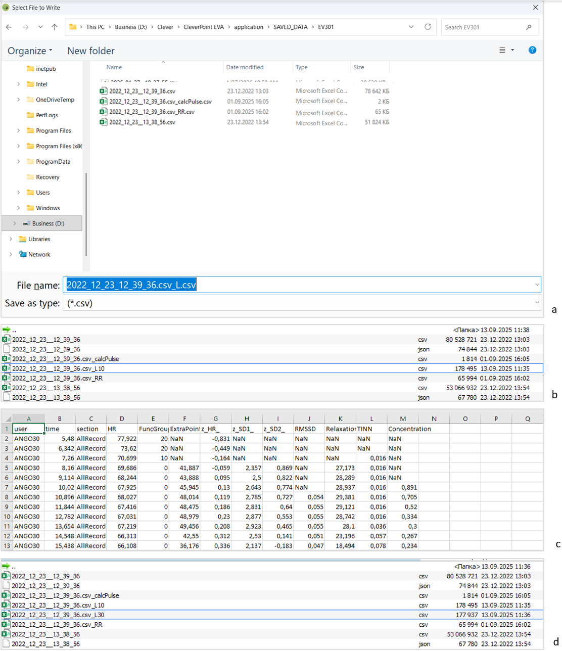
The last functional icon in the form of a floppy disk is also familiar to you: the function of saving data in tabular form. Press it (Fig. 2.29a). You are prompted to save the data under the name of the main file with “_L” added (Fig. 2.29a). Save it. A file with a “tail” in the name “_L10” will appear in the main folder (Fig. 2.29b). 10 is the value of the averaged number active in the window we told you about above. If you select, for example, the value “30” there, then your file will be saved with the “tail” “_L30” in the name (Fig. 2.29d).

Now let us consider how the saved data look in Excel (Fig. 2.29c). Regardless of which graph is activated and which stage is displayed in the sector, the saved file will contain data for all indicators for the entire testing time. Two points that you need to focus your attention on: 1) the functional group is marked on the graph not as 1,2,3 – 9, but as 10, 20, 30 – 90 (this is done for better visualization); 2) if there is no number in a cell and “NaN” is indicated, this means that the indicator could not be calculated at that moment (Fig. 2.29c).

Figure 2.29. Sequence of actions for saving RR-interval data (explanations in the text)

This chapter is perhaps the most difficult, and if you have reached this page, please accept our congratulations!

In the next chapter, we will again work in the “Cardio domain” area, but already in conjunction with the report and examples for analysis and conclusions. The skill of working with “Cardio domain” data is extremely important both for a consultant and for scientific work, unlike other pages of the CleverView program, which are more oriented toward scientific research. Therefore, for now we remain on this page.

Cardio domain: examples

We have already indicated that the “Cardio domain” page is the most illustrative both for the consultant and for the researcher. Now that we are oriented in the page graphs and the ways of controlling the data on it, let us consider these capabilities using specific examples. Click the CleverView program icon; after it loads, immediately activate the “Cardio domain” page and load the file we need.

3.1. ECG recording quality

The first thing that should be paid attention to is the quality of the obtained recording. Figures 3.1, 3.3, and 3.8 present three variants of recording primary data related to the ECG. Let us analyze them.

Figure 3.1 is familiar to you, since the text of Chapter 2 of this manual is built on its example. Therefore, we hope it does not require lengthy explanations. Let us focus only on several points: 1) the need to display the ECG curve in Sector 4 (Fig. 3.1b); 2) pay attention to the shape of the CIG (Sector 5) and to the shape of the scatter-plot clouds outlined by ovals (Sector 7).

Figure 3.1. Example of a high-quality recording (see explanations in the text)

A high-quality recorded ECG in Sector 4 looks like an even palisade. But if the blue background (Fig. 3.1a) of merged lines (we remind you: this is the vertical line marking the detection of the R wave) does not always make it possible to see an ECG complex that has dropped out of the calculation, then the actual ECG curve will not let you make a mistake (an illustrative example in Fig. 3.3).

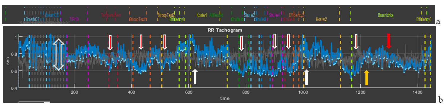
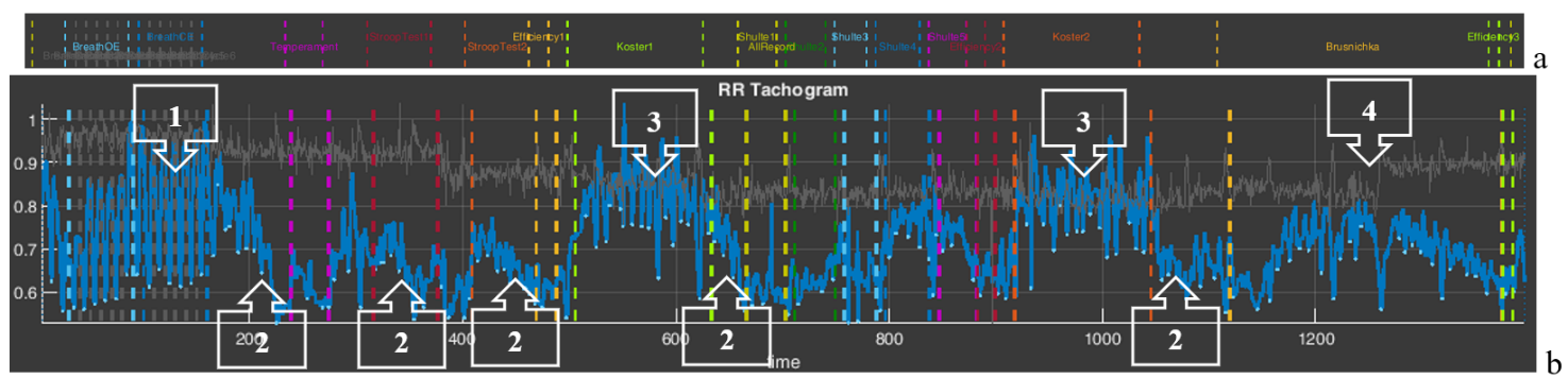
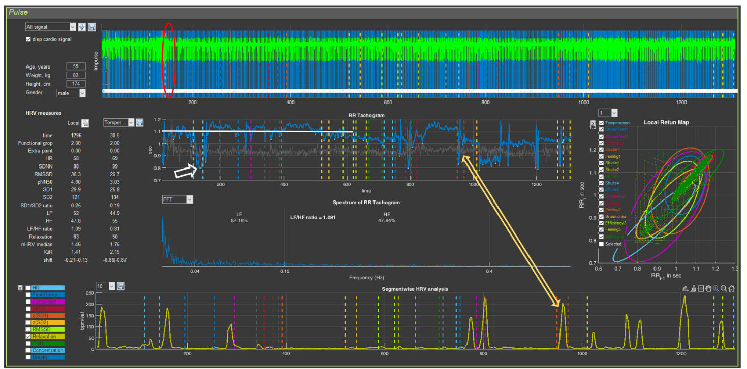
To understand the information about the respondent contained in the CIG, let us recall Fig. 2.18, which we will supplement for clarity with arrows indicating transient processes.

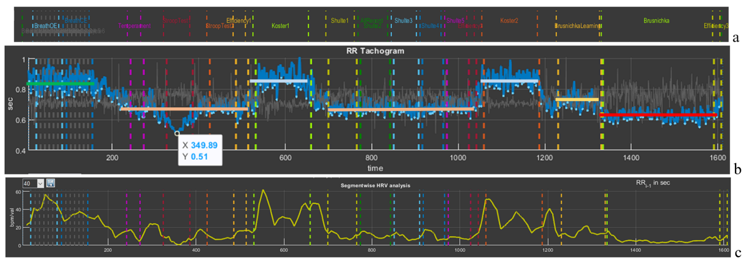
The first thing to pay attention to is the slow-breathing stages at the beginning of the study. This trial pursues several goals: 1) breathing at a rate of about 6 respiratory movements per minute allows a person to adapt to VR conditions and thereby standardize the conditions for everyone when performing subsequent tests in Stressonika. In Fig. 3.2b it can be seen that the HRV amplitude in this test is the largest (the height of the bidirectional vertical arrow); 2) breathing at a rate of about 6 respiratory movements per minute triggers processes of maximum “swinging” of HRV due to activation of the parasympathetic nervous system and, according to one of the approaches to breathing practices, to resonant interaction between the respiratory center and the center controlling the activity of the cardiovascular system in the CNS. This trial makes it possible to see the respondent’s response to such breathing and, consequently, the possibility of recommending to them resonant breathing practice in order to increase parasympathetic tone in situations of emotional tension.

Figure 3.2. Cardiointervalogram for the entire study period (see explanations in the text)

The second observation is fluctuations in RR interval duration that are clearly dependent on the beginning of the testing stages: the vertical red arrows with a white outline directed downward indicate a shortening of the RR interval (and therefore an increase in HR) at the beginning of each test with cognitive load. However, during the 2-minute rest stages (white arrows directed upward), the RR interval duration increases (this is manifested by a decrease in HR). It can be assumed that the beginning of the load tests is stress-inducing for the respondent, but at the same time they are not yet in a state of chronic stress, since, in response to the request to rest during the corresponding testing stages, the body responds adequately by lowering HR. Such a type of response to tests may also indicate the respondent’s emotionality or their involvement in the testing process.

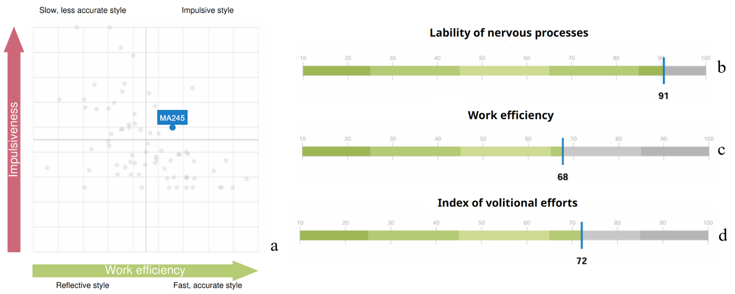
The third observation is the response to the final test, in which cognitive load is combined with a time limit. The respondent’s first reaction is typical for them: at the beginning, HR increases, then decreases (yellow arrow) and the functional state stabilizes for some time, and then (red arrow) HR begins to increase again. This dynamics most likely indicates fatigue. If the productivity of cognitive activity did not decrease by the end of this test, then such a report indicator as the “Volitional Effort Indicator” will be at a sufficiently high level, and vice versa. In this way, the value of the “Volitional Effort Indicator” can be illustrated to the person being consulted using the example of their autonomic response and, consequently, useful recommendations on self-regulation in certain life and professional situations can be given.

We hope that these explanations have shown the benefit of considering the CIG in the format of the entire test. Let us take them as a model for further examples.

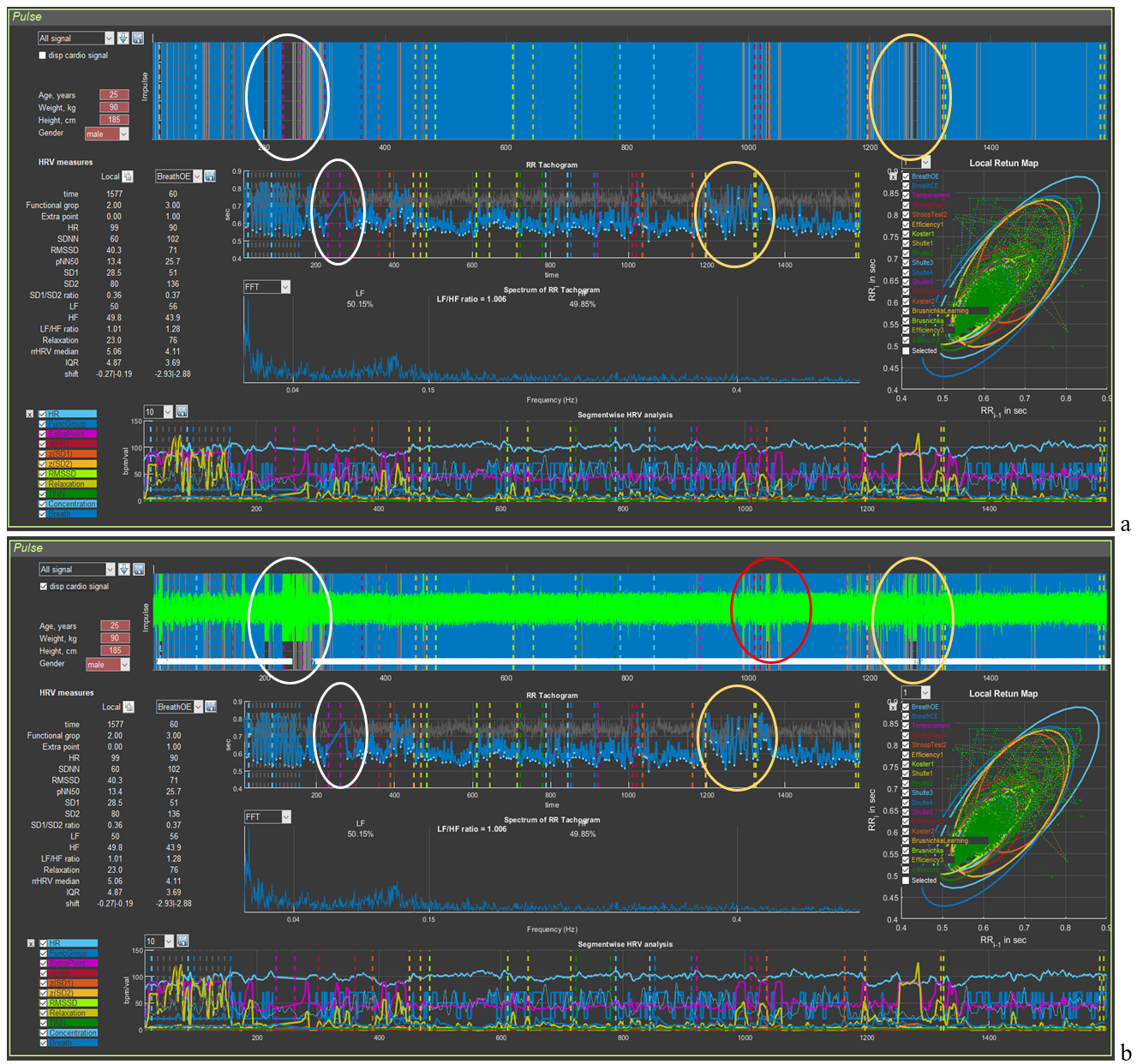
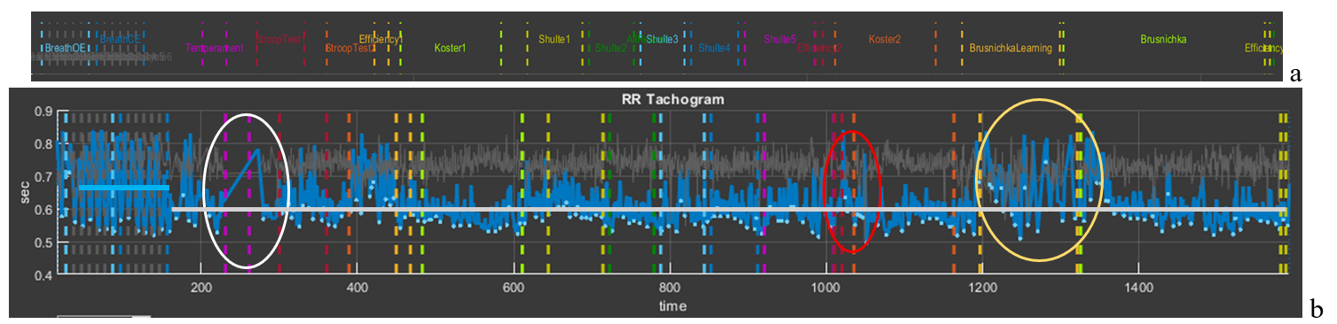
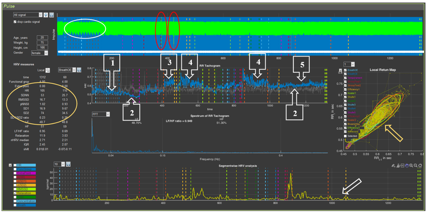
Figure 3.3 presents an example of permissible defects in an ECG recording. Obvious “gaps” between the blue vertical lines (Fig. 3.3a), highlighted by white and yellow ovals, immediately catch the eye. In Sector 5, within this time interval, it can be seen that the CIG structure is disrupted: under the white oval a rather long straight segment is visible, indicating that part of the consecutive ECG complexes were not taken to build the cardiointervalogram curve; under the yellow oval the CIG clearly differs from the general background. If the ECG is additionally visualized in Sector 4 (Fig. 3.3b), other recording defects can also be noticed (highlighted by the red oval). Let us consider these segments in more detail.

Figure 3.3. Example of an acceptable recording (see explanations in the text)

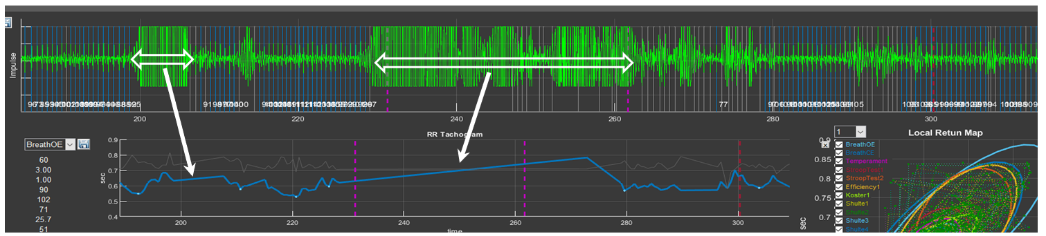
Let us remember the “Zoom In” icon and select the segments marked by the white oval first in Sector 4 and then in Sector 5 (Fig. 3.4). In this time interval, prolonged artifact segments are observed on the ECG (probably related to motor activity), against which identification of the R wave is impossible (the longest ones are marked by horizontal bidirectional arrows). On the CIG, this “failure” in the ECG recording forms a straight segment that connects the recorded RR interval before the artifact begins and the first recorded interval after it (Fig. 3.4). After the longest artifact segment of the ECG recording, other, shorter bursts of artifact activity are also visible, which we hope you can already see on your own.

Figure 3.4. Example of a prolonged artifact ECG recording

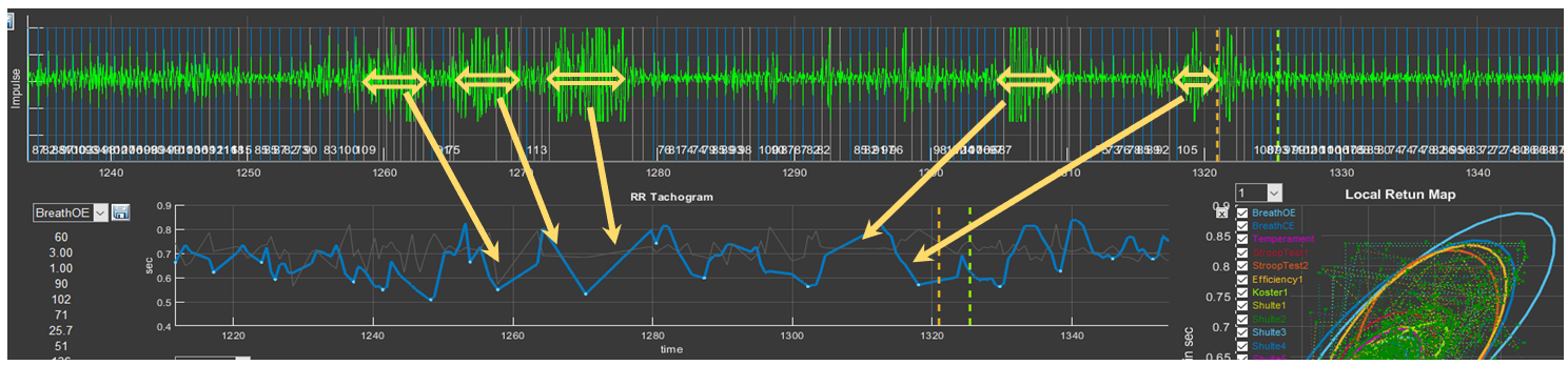
Press the “Restore View” button in Sectors 4 and 5 to restore the initial view of the curves, and then select the segments under the yellow oval (Fig. 3.5). Consecutive short-term artifacts of the ECG recording are visible. In such cases, on the overall CIG curve they look like high-amplitude pointed waves that differ from the general background. When this segment is selected on the CIG curve, short straight segments (indicated by the arrow) can be seen, which are not characteristic of a cardiointervalogram (Fig. 3.5).

Figure 3.5. Example of an ECG recording with consecutive short-term artifacts

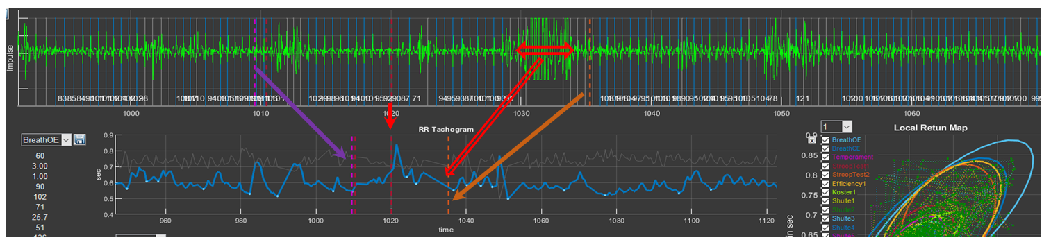
It remains to see what “problems” are present in the ECG recording under the red ovals (Fig. 3.6). Select them and you will see the already familiar picture, with the only difference that the artifacts are brief. Such artifacts, as we hope you have convinced yourself, are better seen when the ECG is activated in Sector 4.

Figure 3.6. Example of an ECG recording with consecutive brief artifacts

Let us answer the question: why is such a recording suitable for analysis and full consultation based on the report? For this, let us refer to Fig. 3.7 (for convenience of perception, in the top line we place a part of the “Time domain” window where the names of the study stages are indicated). Please note that artifact segments are located in zones that are not included in the analysis of the respondent’s psychoemotional state assessment, or when these zones are not critical for holistic perception of the study results: the white oval outlines the stage of becoming familiar with the techniques of controlling the controller in VR; the red oval outlines the period of self-assessment of the effectiveness of performing the Schulte tables; the yellow oval outlines the training stage before testing the last task.

Figure 3.7. CIG for the entire study period acceptable for analysis (see explanations in the text)

If we have decided that the artifacts of the ECG recording are not critical for the overall analysis, let us compare Figs. 3.2 and 3.7. It is striking that the CIG curve in Fig. 3.7 practically lies on one line (highlighted by the gray segment). The RR interval level is determined by the value of 0.6 s or, converted to HR, 100 bpm (tachycardia). At the same time, both during test performance and during rest periods, HR did not change noticeably; i.e., throughout the entire testing period the respondent was in a state of stress. Even during the controlled slow-breathing stage, HR was about 90 bpm (the blue segment illustrating the average RR interval value at this stage), although it can be seen that the CIG range is from 0.55 to 0.82 s, which indicates preservation of the interaction between the centers controlling external respiration and the cardiovascular system, as well as reflex systems determining the tone of these centers.

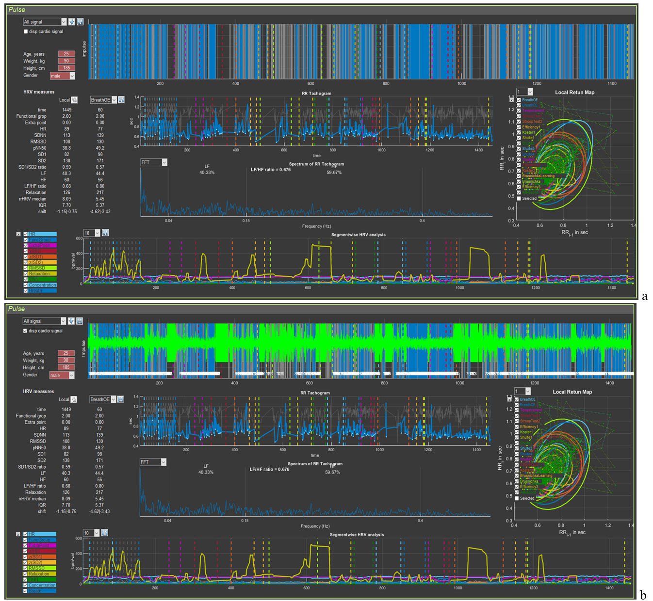
Now an example of a recording unsuitable for assessing the respondent’s psychoemotional state (Fig. 3.8). Upon the initial loading of the person’s file it can be seen that the automatic search for the R wave on the ECG “encounters serious problems”. The palisade of blue lines does not fill the entire space of Sector 4; over the entire recording period, the time of detected R waves (blue color) does not overwhelmingly prevail compared to missed ones (background color) (Fig. 3.8a). Displaying the ECG curve on the screen (Fig. 3.8b) only emphasizes this observation. Zones where registration of the R wave is impossible (intervals filled with artifacts) are present at almost all key stages of testing.

Figure 3.8. Example of a recording unsuitable for analysis of the psychoemotional state (see explanations in the text)

Can the report be commented on in such cases? It can, but only for such sections as: perception, attention, executive functions, efficiency, and properties of the nervous system. That is, for those indicators in which the autonomic response of the person to cognitive stress is not taken into account. But this part of the Stressonika approach is the most important! Therefore, in red letters:

3.2. Preparing the “Cardio domain” page for consultation

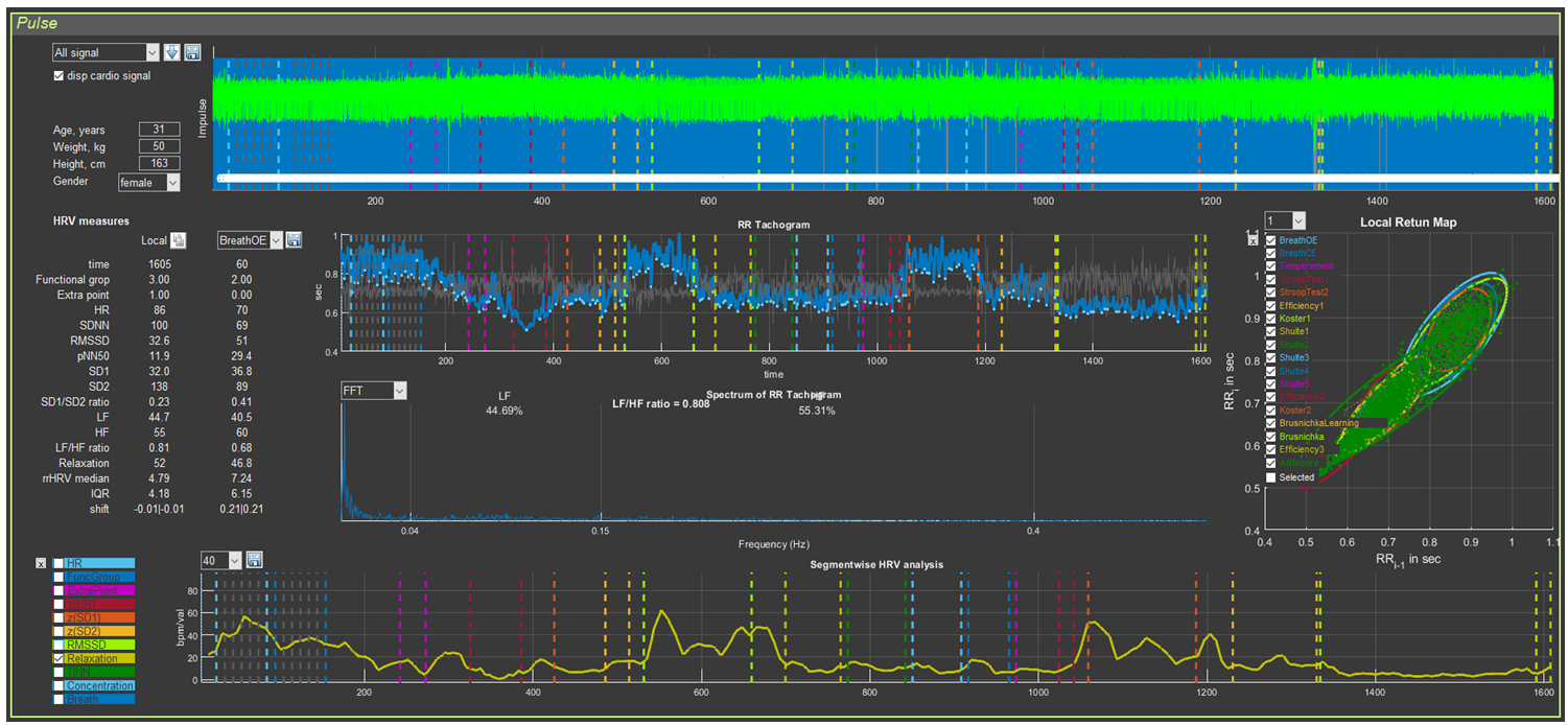
We tactfully yet persistently recommend that you conduct consultation based on the report, emphasizing (illustrating, confirming, accentuating, proving, etc.) your conclusions (reasoning, findings, recommendations, assumptions, etc.) with the respondent’s data displayed on the “Cardio domain” page. Figure 3.9 shows a sample, in our view, of how this page should look for consultation. All subsequent illustrations will correspond to the respondent’s primary data visualized in this figure.

Figure 3.9. “Cardio domain” page prepared for consultation

How the image in Sector 4 is formed has already been discussed. It remains only to clarify the graph of Sector 8. For this, it will be necessary to return to the information in Chapter 2 devoted to this sector (Table 2; Figs. 2.27 and 2.28). From Table 2 it can be seen that, for most indicators, the scientific component predominates. For assessing the respondent’s functional state, the greatest interest is HR (HR on the graph) and the level of relaxation (Relaxation). In Figs. 2.27 and 2.28, a heart-rate graph is shown as an example. However, it was previously stated that the RR interval of Sector 5 is the inverse of HR: the smaller the RR interval (a decrease of the graph in Sector 5), the higher the HR (an increase of the graph in Sector 8), and vice versa. This relationship is illustrated separately in Fig. 3.10. Essentially, these graphs reflect the same thing, being in mirror symmetry. When commenting on the CIG, one rather quickly gets used to speaking in terms of HR. Therefore, displaying the HR graph separately in Sector 8 is of little informative value, unlike the relaxation dynamics graph, which we recommend using during consultation.

Figure 3.10. Interdependence of the graphs of Sector 5 and Sector 8 if heart rate values are displayed on the latter

To display the relaxation dynamics graph as shown in Fig. 3.9, a number of manipulations should be performed, which are described in Chapter 2 in the corresponding advisory section: reset all graphs, activate the “Relaxation” graph, scale vertically, and smooth (if necessary) by the number of averaged points of the recorded primary data (in our example, 40 points).

We have prepared the “Cardio domain” page, opened the report, and are now ready for consultation.

3.3 Viewing the “Cardio domain” page during consultation (Example 1)

Our first example will be the visualized biometric data shown in Fig. 3.9.

The first thing to pay attention to before starting the consultation is assessment of the recording quality (see above). In Sector 4, a sufficiently high-quality ECG recording is observed, which makes it possible to draw conclusions for the entire report.

The second thing to which we recommend paying attention is the anthropometric data (Sector 2). We see: age 31 years, female, weight 50 kg, height 1.63 m. The body mass index (BMI) can be calculated ≈ 18.8. The BMI value is rather significant information (Table 3.1) that may be useful during consultation.

Table 3.1. Body mass index and its assessment

Now you can proceed to the description of the report.

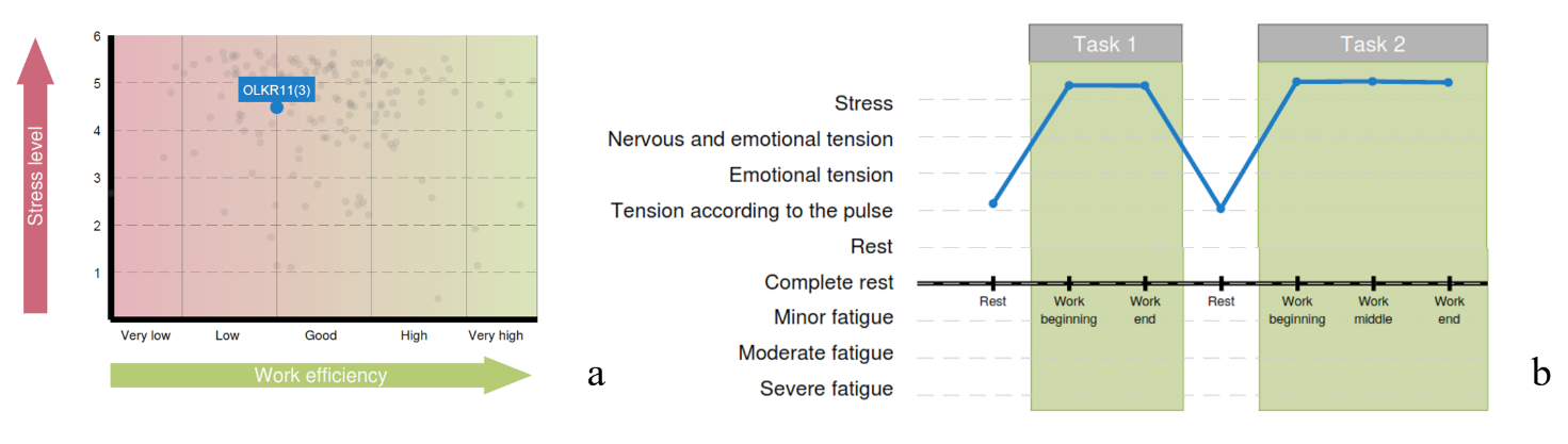
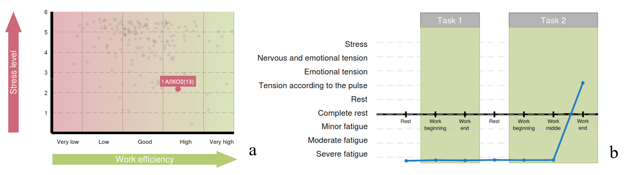
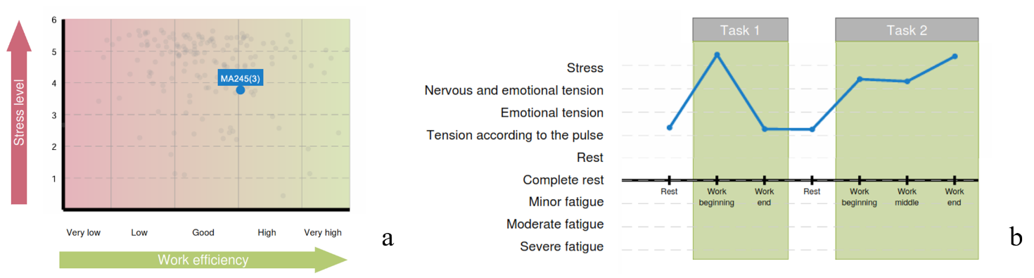
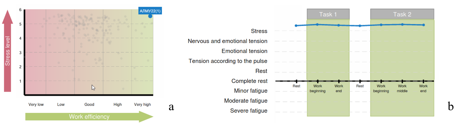
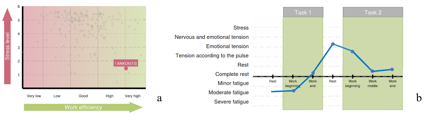
Chapter 3 of the report is the one most closely related to the “Cardio domain” page. Two diagrams of Chapter 3 of the respondent’s report, whose primary data were taken by us as the first example, are presented in Fig. 3.11. For assessing the respondent’s psychoemotional state and their individual reaction to stress, these diagrams are the most important.

Figure 3.11. Diagrams of Chapter 3 of the report: a – functional type of work capacity support; b – functional states of the respondent in the process of performing test tasks

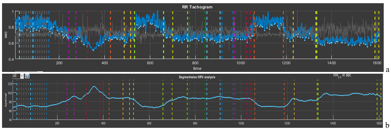
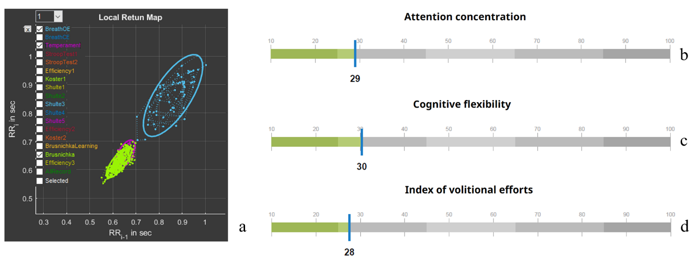
Let us begin with the diagram “Functional type of work capacity support” (Fig. 3.11a). Note the rather high position on the “Stress level” scale, the borderline position between “low” and “good” on the “Work efficiency” scale, and the blue fill color of the respondent’s position mark on the diagram. In the diagram “Functional states of the respondent in the process of performing test tasks”, the intensity of the psychoemotional state during testing in Stressonika and its dynamics are already indicated in terms of certain functional states (Fig. 3.11b). The diagram clearly shows that during the 2-minute periods of the proposed rest the respondent was able to return to a state adequate to the test conditions at those moments. On the CIG curve of the “Cardio domain” page (Fig. 3.12), this dynamics is only confirmed: during all periods of cognitive tests the respondent was in a state of stress, as indicated by a decrease of the CIG or an increase in HR (pink and red segments), and it increases during rest periods (blue segments). Note that both tension and rest states are quite stable: RR intervals, with the exception of the StroopTest1 period, where a sharp increase in HR is visible (RR interval = 0.51 s, which corresponds to HR = 117.6 bpm), fluctuate approximately within the same range (Fig. 3.11b). To understand the difference between mobility and stability of heart rhythm, let us compare Figs. 3.2 and 3.11b.

Figure 3.12. Interdependence of the graphs of Sector 5 and Sector 8 if heart rate values are displayed on the latter

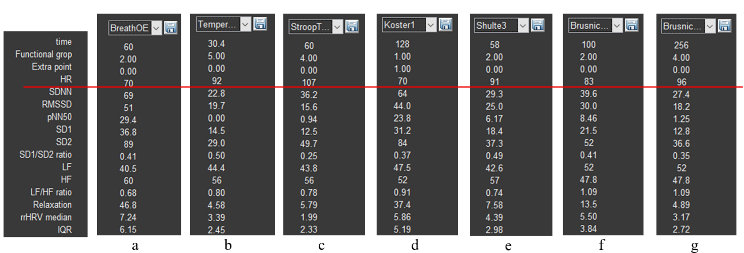
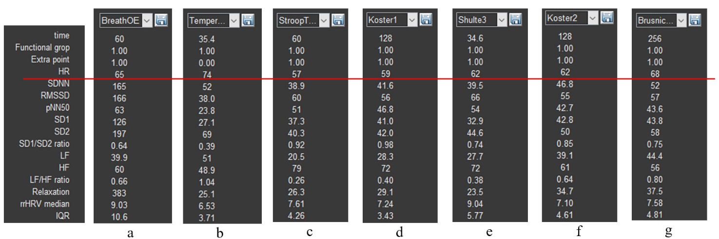
The ability to return to a state of relative rest (we remember that “
rest is only a dream”) after tension is a remarkable quality of an individual, which indicates the absence of chronic stress and/or a balance of the sympathetic and parasympathetic nervous systems. It is not by chance that the fill color of the respondent’s position on the diagram “Functional type of work capacity support” is blue. Figure 3.12c, reflecting the dynamics of relaxation intensity, only emphasizes what has been described above. Your reasoning about HR can be supported by the data of Sector 3 if HRV data of a particular testing stage are displayed in the right column (Fig. 3.13). In the figure, HR data are highlighted by a red stripe; the data above it, already in digital form, consolidate our observations.

Figure 3.13. HRV indicators: a – controlled slow-breathing stage with eyes open; b – tapping test stage; c – Stroop test 1 stage; d – first rest stage; e – Schulte table 3 stage; f – training stage for the color test with names of fruits and vegetables; g – stage of performing the color test with names of fruits and vegetables.

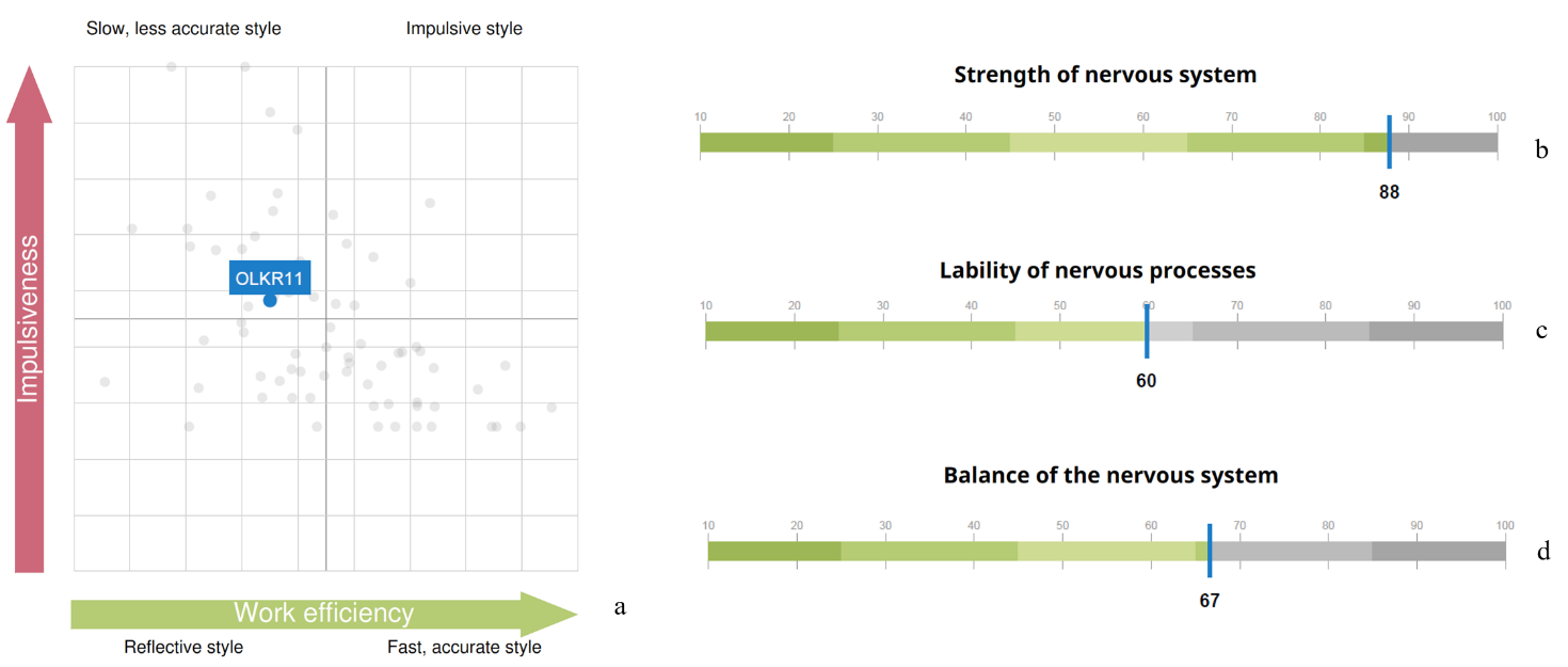
The third diagram of Chapter 3 of the report reflects the respondent’s cognitive style (Fig. 3.14a). The tested individual’s position falls into the “Slow inaccurate style” zone. Let us remember that during test performance our participant was in a state of stress. This allows the conclusion that this state is not the most productive for their cognitive activity. Methods of emergency workload or brainstorming are not their element.

Figure 3.14. Graphs of Chapters 3 and 4 of the report: a – cognitive style diagram; indicators of nervous system strength (b), mobility (c), and balance (d)

It can be assumed that the results presented in Chapter 4 of the report – “Properties of the nervous system” (Fig. 3.14a,b,c) – are reflected in the CIG pattern: the ability to maintain such a functional state as stress at the same level for a long time – strength of the nervous system; the ability to quickly switch from a state of stress to “pulse tension” – mobility; a sufficiently wide band of RR interval fluctuations, as well as some HRV indicators (e.g., SD1/SD2) – balance.

In addition to the report, the respondent can also be told about other observations.

1. Even during testing it was noticeable how the respondent emotionally reacted to the last test. In Fig. 3.12b this stage is highlighted by a red segment that is clearly lower than other parts of the CIG, which confirms the tested person’s involvement in the process of the assigned tasks. Highlighting the RR-interval distribution cloud in Sector 7 of this stage (bright green) in comparison with the slow-breathing task (blue), which models a rest state, clearly shows that the cloud of the last test is located markedly lower and occupies a smaller area (Fig. 3.15a). This location and shape indicate activity of the sympathetic nervous system, which is manifested by an increase in HR and a decrease in HRV.

Figure 3.15. a – scatter plot (Sector 7); report indicators of attention concentration (b), cognitive flexibility (c), and volitional effort (d)

At the same time, now in concrete numbers (Fig. 3.15b,c), indicators of cognitive functions are below average values. Thus, involvement in the last test did not affect the overall assessment of these indicators and did not influence efforts to overcome the fatigue factor at the end of the test (Fig. 3.15d). It has already been concluded that a state of stress is not the best one for the respondent’s work performance. Even under a positive emotional background, the style of work under stress is more reminiscent of fussiness.

2. A rather important stage is the first two tasks of controlled slow breathing. In subsection 3.1 of this chapter, the significance of this functional trial has already been discussed. Therefore, it is desirable to discuss the data of the “BreathOE” and “BreathCE” stages with the respondent. Activate in Sector 1 the stage with eyes open (OE) (Fig. 2.3b), select (following the example in Fig. 2.5b, but in Sector 5) this stage on the CIG, and in Sector 7 activate the stages “BreathOE”, “Koster1”, and “Temperament” (Fig. 3.16).

In Sector 5, a time range of 1 min is selected (Fig. 3.16a). On the CIG curve, 9 waves of sinusoid-like oscillations of RR intervals are visible, i.e., 9 per minute. Such a shape indicates that these oscillations occurred in accordance with respiratory movements. On the spectrogram in such cases, a peak is clearly visible whose frequency value corresponds to the number of waves on the cardiointervalogram (Fig. 3.16b). Let us check: the peak frequency is 0.152 Hz, which, converted to the number per minute, is 0.152 * 60 = 9.1. We remember that, according to the instruction, the respondent was supposed to breathe at a rate of 6 respiratory movements per minute. The same pattern was observed at the stage with eyes closed – “BreathCE”. There is a topic for discussion: why the respondent breathed at a different rate. Possibly they did not understand the instruction, due to discomfort or for some other reason; perhaps breathing practices are not suitable for the respondent as training tools for achieving a state of relaxation.

Figure 3.16. “BreathOE” stage on the “Cardio domain” page prepared for consultation

Be that as it may, respiratory arrhythmia is clearly visible on the CIG, i.e., correspondence of changes in RR interval values to the phases of respiration: inhalation/exhalation. More often such correspondence is observed in a rest state; therefore, the form (cloud) of the RR-interval distribution in Sector 7 can be taken as a comparison state with other stages (blue color), for example, the rest period (bright green) and the “Temperament” stage (violet), which most often is supported by the maximum activity of the sympathetic nervous system (Fig. 3.16c).

3. Now the first rest stage can be considered in more detail (Fig. 3.17). On the CIG (we remember that this stage lasts 2 min) signs of respiratory arrhythmia are observed, but not as organized as it was during the “BreathOE” stage (Fig. 3.17a). The fact that at this stage there is no clear relationship between respiration and RR-interval oscillations is also confirmed by the absence of a pronounced peak on the spectrogram (Fig. 3.17b). However, the RR-interval distribution “cloud” (bright green) almost exactly coincides with the cloud of the controlled breathing period. It can be concluded that at this time the respondent was in a state of relative rest, which has already been stated when discussing the report.

Figure 3.17. “Koster1” stage on the “Cardio domain” page prepared for consultation

Based on the first example, perhaps one more emphasized remark can be made: Stressonika does not assess the level of intelligence, and low indicators of cognitive functions are not a reason for sharp and unambiguous conclusions. The database on which the indicator scales in the report are built is a range of normal values! The task of Stressonika: assessment of a person’s functional state, burnout risk, ability to perform cognitive tasks under stress, identification of individual characteristics of a person’s response in a state of emotional tension, provision of objective data for self-knowledge, revealing to a person their strong and weak properties of the body’s functioning, development of strategies for optimal performance of tasks at work and in everyday life, and restoration of the balance of internal mechanisms that determine the quality of our life.

We hope that the first example was sufficiently useful for understanding the philosophy embedded in Stressonika.

3.4 . Viewing the “Cardio domain” page during consultation (Example 2)

So that you do not form a superficial impression that stress and burnout revolve only around tachycardia, let us consider one more example (Fig. 3.18).

Figure 3.18. The respondent’s “Cardio domain” page (Example 2)

The first thing we pay attention to is the quality of the ECG recording. It is good, which allows us to draw conclusions not only from the report as a whole, but also from the data of the respondent’s autonomic reaction to Stressonika. The second point of our attention is the cardiointervalogram (Fig. 3.19b).

Figure 3.19. The respondent’s cardiointervalogram (CIG) acceptable for analysis (Example 2).
Note: a – an element of the “Time domain” page describing the testing stages in Stressonika.

What catches the eye on the CIG curve:

1. a relatively low heart rate (HR), which is fairly stable throughout the entire testing time (the red line of the mean RR-interval duration is approximately at the level of 0.95 s, or, converted to HR, 63 beats/min);
2. a wide spread of RR intervals at the breathing stages (the vertical bidirectional arrow);
3. a certain increase in HR during the tapping test and during the last test, up to 60/0.8 = 75 beats/min;
4. a decrease (!) in HR in response to the Stroop test and during the first 2-minute rest.

Let us check our observations against specific numbers using Sector 3 (Fig. 3.20).

Figure 3.20. HRV indicators (Example 2): a – the stage of controlled slow breathing with eyes open; b – the tapping-test stage; c – the Stroop test 1 stage; d – the first rest stage; e – the stage of completing Schulte table 3; f – the second rest stage; g – the stage of completing the color test with names of fruits and vegetables.

The range of RR-interval duration at the controlled breathing stage with a frequency of 6 breathing movements is quite large, and the CIG clearly shows relatively rare oscillations of the cardiac cycle duration organized into a certain rhythm. However, we recommend always viewing this stage in CleverView. We remind you how to do this: in Sector 1, activate the slow breathing with eyes open stage that we need (this action will display the spectrogram of this stage in Sector 6; see Fig. 3.21b); in Sector 7, visualize only the “BreathOE” stage (Fig. 3.21c); in Sector 5, stretch the part of the CIG curve highlighted with a thicker line (Fig. 3.21a). The resulting image on the “Cardio domain” page is a clear example of why such a detailed analysis of the respondent’s response to the controlled slow breathing stage is necessary!
Let us sort it out.

Figure 3.21. The respondent’s “BreathOE” stage (Example 2): a – cardiointervalogram; b – spectrogram; c – scatter plot

The cardiointervalogram curve clearly illustrates that the respondent was able to “pick up” the imposed breathing only in the second half of the “BreathOE” stage (in Fig. 3.21a, the area under the white oval), while at the beginning the breathing was more frequent (the CIG under the yellow oval in Fig. 3.21a). On the spectrogram, this moment is reflected by two corresponding peaks (Fig. 3.21b). The slow breathing with eyes closed stage (Fig. 2.22) emphasizes the nuance that it was more comfortable for the respondent—which was confirmed in the conversation after testing—to breathe at a higher frequency. On the spectrogram, only one peak at a frequency of 0.137 stands out, which corresponds to ≈ 8 breathing movements. These data may be useful when selecting individual approaches to certain breathing practices.

Figure 3.22. The respondent’s “BreathCE” stage (Example 2): a – cardiointervalogram; b – spectrogram; c – scatter plot

Moving on. The response on the part of cardiac activity (by the shape of the CIG) is not quite usual for Stressonika. Let us compare it with the results of the report (Fig. 3.23).

Figure 3.23. Diagrams of Chapter 3 of the report (Example 2): a – the functional type of performance support; b – the respondent’s functional states in the process of performing test tasks

A red zone with a low level of stress reaction severity (Fig. 3.23a) and a state of pronounced fatigue almost throughout the entire session (Fig. 2.23b). It can be assumed that the respondent’s functional state does correspond to what was identified in Stressonika, despite the respondent’s lack of complaints of fatigue. There are no contradictions in this combination, since the level of stress is most often determined by heart rate, but an HR at the level of 60 beats/min can be the result of activation of the protective parasympathetic nervous system against the background of chronic stress. To confirm this assumption, one of the rest stages can be considered in more detail, for example “Koster1” (Fig. 3.24).

Figure 3.24. The respondent’s “Koster1” stage (Example 2): a – cardiointervalogram; b – spectrogram; c – scatter plot

On the CIG (Fig. 3.24a), there are no signs of respiratory arrhythmia, which should be observed in the case of balance between the sympathetic and parasympathetic nervous systems. On the spectrogram (Fig. 3.24b), there is a pronounced shift of spectral power toward high (HF) frequencies—70.28%. The scatter plot (Fig. 3.24c) forms not even an oval, as happens when the structures of the autonomic nervous system are balanced, but rather a circle, the conventional width (bidirectional arrows) of which corresponds to the SD1 indicator. These same indicators are present in the table of Sector 3 (Fig. 3.20d). Let us refer to Table 2.1 of Chapter 2: HF is a measure of the power of high-frequency influences of neurohumoral regulation, which is associated mainly with the parasympathetic link of regulation; SD1 reflects instantaneous changes in RR-interval duration, also related to the activity of the parasympathetic division of the ANS. The assumption of parasympathetic dominance is confirmed.

It can be concluded that the respondent’s organism, in response to the chronic stress in which they are at the time of testing, has reorganized to a different mode of functioning, in which increased activity of the parasympathetic division of the ANS is clearly traced. This is a protective adaptive reaction, which also influences the absence of formation of a feeling of fatigue.

3.5. Viewing the “Cardio domain” page during consultation (Example 3)

And now let us consider CleverView data of a respondent who complains of chronic fatigue (Fig. 3.25).

Figure 3.25. The respondent’s “Cardio domain” page (Example 3)

Recording quality? There are problems (Fig. 3.25): a segment of the recording defect on the last test is highlighted by a vertical oval, and single defects at the rest stages and Schulte tables are highlighted by a horizontal oval. A detailed analysis showed that these problematic segments of the recording do not have a significant effect on the overall picture.

For clarity, let us present the CIG in a separate image and mark the zones of our attention (Fig. 2.26): 1 – during controlled rare breathing, high-amplitude waves of respiratory arrhythmia are clearly visible; 2 – a mobile reaction to the beginning of various psychometric tests with an HR shift toward tachycardia (up to 100 beats/min); 3 – during the proposed rest periods, recovery of a more slowed rhythm of heart contractions is noted (down to 70 beats/min); 4 – the cardiac-rhythm reaction during the last test is similar to that described at the beginning of this chapter (see Fig. 3.2).

Figure 3.26. The respondent’s CIG acceptable for analysis (Example 3).
Note: a – an element of the “Time domain” page describing the testing stages in Stressonika.

1. Slow breathing, especially with eyes closed (Fig. 3.27), exactly corresponds to the set rhythm. The shape of the CIG during respiratory arrhythmia (Fig. 3.27a) and the scatter plot (Fig. 3.27c) are close to optimal.

Figure 3.27. The respondent’s “BreathCE” stage (Example 2): a – cardiointervalogram; b – spectrogram; c – scatter plot

2. Mobility of nervous processes, according to the report (Fig. 3.28b), is high, which is emphasized by the autonomic reaction to the beginning of cognitive tests and the identified cognitive style (Fig. 3.28a). At the same time, work performance is above average (Fig. 3.28c).

Figure 3.28. Graphs from the report (Example 3): a – cognitive style diagram; b – nervous system mobility; c – work performance; d – volitional effort indicator

3. During the rest periods, HR decreases, which is illustrated by the mean level of the CIG (Fig. 2.29a). The arrows (Fig. 2.29a,c) indicate segments with R waves that were not recognized (see comments to Fig. 3.25 and Fig. 3.5), which, however, weakly affects the overall background of the cardiointervalogram curve. At the same time, signs of respiratory arrhythmia can be noted both on the CIG itself and on the spectrogram in the form of a distinct peak (Fig. 3.29b).

Figure 3.29. The respondent’s “Koster1” stage (Example 3): a – cardiointervalogram; b – spectrogram; c – scatter plot

4. A high volitional effort indicator (Fig. 3.28d) indicates that, despite the signs of fatigue that were observed during the last test, the respondent is able to concentrate on the assigned task and bring it to completion.

The impression is created that the respondent is not in a state of chronic stress. This is also confirmed by the information of Chapter 3 of the report (Figs. 3.30 and 3.28a).

Figure 3.30. Diagrams of Chapter 3 of the report (Example 3): a – the functional type of performance support; b – the respondent’s functional states in the process of performing test tasks

However, the conclusions we have made do not at all mean that the respondent should not complain of fatigue. We can only assume that the cause of these complaints is not a state of chronic stress. It is possible that such a type of response to a stressor, with a relatively low strength of the nervous system (according to the report), under the “pressure” of volitional efforts, leads to short-term but frequent states of fatigue. In addition, besides chronic stress, there are many other reasons that can form such a sensation. This needs to be dealt with. But this is already a problem that lies outside the scope of this manual.

3.6 . Viewing the “Cardio domain” page during consultation (Example 4)

Let us give another example of an excessive autonomic reaction to completing the battery of tests in Stressonika (Fig. 3.31).

The quality of the ECG recording is good for almost the entire time (with the exception of short-term defects highlighted in the figure by red ovals), which gives us the opportunity to rely on the HRV indicators calculated by the CleverView program during the consultation based on the report.

Figure 3.31. The respondent’s “Cardio domain” page (Example 4)

With a holistic perception of the “Cardio domain” page, the following points can be highlighted: 1. a state of pronounced anxiety, which manifested already at the beginning of the test and persisted throughout the VR session in the form of tachycardia (see the HR values in Fig. 3.31 in Sector 3); 2. extremely low heart rate variability, which manifests as a narrow shape of the CIG, elongated ovals of the scatter plots (yellow arrow) and is emphasized by the HRV indicator values (highlighted by a yellow oval in the figure); 3. an uncharacteristic reaction in the form of a slowing of the heart rhythm during the performance of a test associated with cognitive tension; 4. during the rest stages, HR decreases, but does not reach values characteristic of the norm (the mean cardiac-cycle duration is about 0.65 s, which corresponds to 92 beats/min); 5. during the last test, the respondent’s functional state stabilized, but at the level of about 100 beats/min. All this logically fits into the extremely low values of such an indicator as the rest state (in Fig. 3.31 in Sector 8 it is indicated by a white arrow).

Let us consider in more detail the stage with controlled slow breathing (Fig. 3.32).

Figure 3.32. The respondent’s “BreathCE” stage (Example 4): a – cardiointervalogram; b – spectrogram; c – scatter plot

The slow breathing proposed in Stressonika should “swing” HRV. However, in our example, the range of RR-interval values is extremely modest (Fig. 3.32b). At the same time, such indicators as the position of the spectrogram peak along the horizontal axis in the zone corresponding to 6/min (Fig. 3.32c) and the dynamics of the R-wave amplitude (Fig. 3.32a), which is more clearly illustrated by the R-wave envelope (the gray line in Fig. 3.32b), indicate that the respondent was breathing in the rhythm set in the test. Consequently, the low HRV values can be associated with excessive activity of the sympathetic nervous system, and the respondent’s state can be assessed as stress.

The reaction in the form of a slowing of the heart rhythm during the performance of a test associated with cognitive tension also indicates excessive anxiety from the testing procedure itself. In such cases, completing the test becomes a push toward a more balanced emotional response.

Let us look into the report (Fig. 3.33). CleverView information is an excellent illustration of the information that is formed in the report, only not in terms that are not always clear to the respondent, but in indicators of their individual bodily reaction. We note high work efficiency against the background of a pronounced stress reaction and the blue background of the personal marker. Our respondent is among that cohort of people for whom stress is a stimulating background for successful work. Will they be able to work productively for a long time in such a mode? The question is rather rhetorical.

Figure 3.33. Diagrams of Chapter 3 of the report (Example 4): a – the functional type of performance support; b – the respondent’s functional states in the process of performing test tasks

One can also look into Sector 2 of the “Cardio domain” page. 20 years old, BMI = 27.2. Is there something to discuss with the respondent? Of course!

3.7. Viewing the “Cardio domain” page during consultation (Example 5)

This example will begin with the report data (Fig. 3.34). This is exactly the case when, without raw data, it is impossible to conduct a full consultation based only on the report.

Let us deal with Example 5.

Here the situation is rather confusing: high work efficiency with a low stress level, but the respondent is in the red zone; the functional-state graph begins with moderate fatigue, and the state with the highest tension occurs during the second rest, while the cognitive load was performed in the rest zone, which is difficult to expect during the performance of test tasks.

Figure 3.34. Diagrams of Chapter 3 of the report (Example 5): a – the functional type of performance support; b – the respondent’s functional states in the process of performing test tasks

Let us look at the “Cardio domain” page (Fig. 3.35). What draws attention: pronounced fairly stable bradycardia, with HR fluctuations from 54 (highlighted by a white line in the figure) to 75 beats/min (white arrow); a narrow CIG curve, which indicates low heart rate variability (this is confirmed by the data of Sector 3); red vertical lines (under the red vertical oval in the figure) in Sector 4, with which the CleverView system marks possible extrasystoles (we select this segment and make sure (Fig. 3.36) that some marks identified premature heart contractions correctly); age—59 years with signs of excess body weight—BMI = 27.4; spikes of rest periods are artifacts associated with defects of the ECG recording (yellow arrow).

Figure 3.35. The respondent’s “Cardio domain” page (Example 5)

Figure 3.36. Premature heart contraction—extrasystole (Example 5)

Conclusion: signs of chronic stress with depletion of reserves (in contrast to Example 2) for maintaining an optimal state of the organism, with preserved high cognitive function. Considering the respondent’s age, their attention should be drawn to the need to monitor their health status and to turn to practices for maintaining mental and physical health in order to replenish reserves and reduce the pressure on the organism of the state of chronic stress.

Using Example 5, let us illustrate one more possible option for using Sector 8. In Fig. 3.37, this sector reflects the dynamics of the respondent’s functional state throughout the entire testing time. For some, this function may be more visually clear than the rest-level curve. For those who will use this curve, some clarifications and recommendations:

1. the averaging value should be set to at least 50 (we remind: the window for selecting the averaging measure is under the white oval;
2. the vertical-value scale is from 0 to 100;
3. vertical scale values for the functional state indicator: 0 – “Complete rest”; 10 – “Rest”; 20 – “Pulse-based tension”; 30 – “Emotional tension”; 40 – “Nervous-emotional tension”; 50 – “Stress”; 60 – “Mild fatigue”; 70 – “Moderate fatigue”; 80 – “Pronounced fatigue”.

Figure 3.37. Dynamics of the functional state (Example 5)

The functional-state dynamics graph can be compared with Fig. 3.34b. It is obvious that the curve in Fig. 3.37 is more detailed.

P.S.
The study result and the conclusions made “impressed” the respondent and pushed them toward the need to “help” their organism. The approaches they chose in this direction yielded their results (Fig. 3.39).

Figure 3.38. The respondent’s “Cardio domain” page after 7 months (Example 5)

Try to draw the conclusions that can be made from the presented figure in comparison with the initial state yourself.

3.8. The “Cardio domain” page. Conclusion.

The information of the report and the raw CleverView data provide a wide field for communicating with the respondent about the features of their response to a situation of uncertainty, organization of personal activity, methods of self-knowledge and self-management, and many other aspects. We hope that we have managed to convince you of this with the help of the examples described in this chapter.

We emphasize that these are only examples, not templates! We remind you that you will not find two identical curves, graphs, and diagrams—each individual is unique! Yes, with experience, some common features will be visible in certain testing results and recorded physiological indicators. This will facilitate analysis of the obtained data and your communication with the respondent. But this will come only with experience, which still needs to be acquired! You will not acquire it if your work with CleverPoint is limited only to a single report without its support by the data of the “Cardio domain” page of our CleverView software product.

Perhaps you will find some of your own methods and approaches to working with the “Cardio domain” page. We do not limit you to our approaches.

Overcoming difficulties begins with the most difficult—the first step! To the extent of our capabilities, we tried to make easier this beginning of your movement to new heights in your profession.

Good luck!