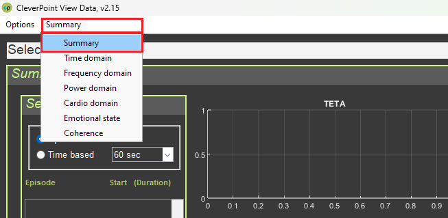
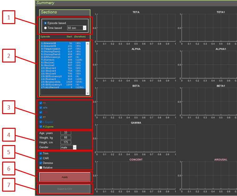
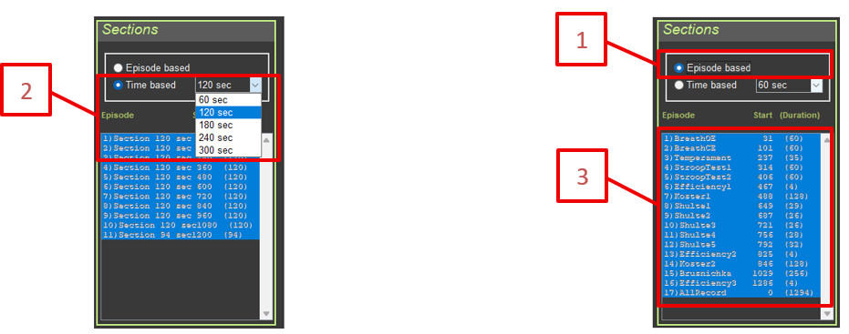
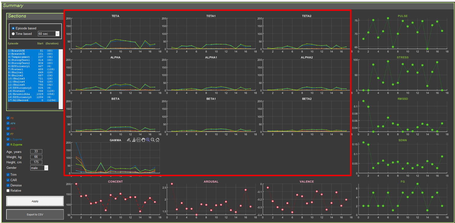
CleverPoint View is a desktop research tool for analyzing multichannel physiological recordings (EEG-like channels plus cardio/ECG) in the context of experimental sessions. The program reads data from CSV files, splits the recording into sections (episodes), applies standard cleaning and filtering procedures, and displays the results on several thematic screens.
The interface is focused on quickly reviewing signal dynamics over time, spectral characteristics, inter-channel relationships, heart rate variability metrics, and simple “emotional state” indices. These indices are not diagnostic; they are simply computed using the formal formulas described below.
This guide describes the functionality of all application interfaces and provides detailed explanations of the signal transformations for psychophysiology researchers.
0. Fundamentals of Electrophysiology for Beginners
0.1. What Are Physiological Signals?
Physiological signals are electrical potentials generated as a result of the activity of living tissues. This application analyzes three main types of signals:
0.1.1. EEG (Electroencephalogram)
Physiological basis: EEG records the electrical activity of the cerebral cortex. This activity arises from synchronized changes in the membrane potentials of large groups of neurons (pyramidal cells).
How it works:
Neurons generate electrical potentials when transmitting information.
When thousands of neurons become active synchronously, their potentials sum together.
Electrodes on the surface of the head record these summed potentials.
The signal amplitude is typically 10–100 microvolts (µV).
What EEG shows:
General brain state (wakefulness, sleep, coma)
Cognitive processes (attention, memory, thinking)
Emotional states
Pathological changes (epilepsy, tumors)
EEG frequency ranges (and their physiological meaning):
Delta (0.5–4 Hz): Deep sleep, pathological conditions, infancy
Alpha (8–13 Hz): Relaxed wakefulness with eyes closed, calm state
Beta (13–30 Hz): Active thinking, concentration, problem solving
Gamma (30–100 Hz): High-level cognitive processing, binding information from different brain areas
0.1.2. ECG (Electrocardiogram)
Physiological basis: ECG records the electrical activity of the heart. Each heartbeat (systole) is initiated by an electrical impulse that propagates through the heart’s conduction system.
How it works:
The sinoatrial node (the pacemaker) generates an electrical impulse.
The impulse spreads through the atria to the atrioventricular node and then to the ventricles.
Electrodes on the body record these electrical changes.
The R-peak in the ECG corresponds to ventricular depolarization (contraction).
What ECG shows:
Heart rate (pulse)
Rhythm regularity
The state of the cardiac conduction system
Heart rate variability (HRV), an indicator of autonomic regulation
Heart rate variability (HRV):
A healthy heart does not beat like a metronome—intervals between beats constantly change.
This variability is controlled by the autonomic nervous system.
High variability = good adaptability and health.
Low variability = stress, fatigue, and possible health problems.
0.1.3. EMG (Electromyogram)
Physiological basis: EMG records the electrical activity of muscles. When a muscle contracts, muscle fibers generate electrical potentials.
How it works:
Motor neurons send signals to muscle fibers.
Muscle fibers depolarize and contract.
Electrodes on the skin record this activity.
In this application, EMG is recorded from facial muscles (Zygoma — cheek muscles).
What EMG shows:
Muscle tension
Facial reactions (smile, grimace)
Stress and emotional reactions (facial muscle tension)
0.2. Autonomic Nervous System (ANS)
The autonomic nervous system controls involuntary body functions, including heart rhythm, breathing, and digestion.
Two branches of the ANS:
Sympathetic nervous system (“fight or flight”):
Activated during stress, danger, or physical exertion
Increases heart rate
Reduces heart rate variability
Prepares the body for action
Parasympathetic nervous system (“rest and digest”):
Activated during rest and relaxation
Decreases heart rate
Increases heart rate variability
Promotes recovery and rest
ANS balance:
A healthy body maintains a dynamic balance between the sympathetic and parasympathetic systems.
HRV analysis makes it possible to assess this balance.
Impaired balance may indicate stress, fatigue, or disease.
0.3. Emotions and the Brain
Valence–arousal model:
Valence: Positive or negative evaluation of an emotion (pleasant/unpleasant)
Arousal: Level of activation (calm/excited)
Hemispheric asymmetry:
Left hemisphere (AF3): Associated with positive emotions, approach behavior, and activity
Right hemisphere (AF4): Associated with negative emotions, avoidance, and caution
Frequency patterns of emotion:
Alpha activity: Relaxation, calmness
Beta activity: Active thinking, stress, anxiety
Beta/alpha ratio: Level of activation/arousal
0.4. Electrodes and Their Placement in the CleverPoint Setup
10–20 system (standard EEG electrode placement)
Variant 1: Reference electrode at Fz. Unipolar connection.
Variant 2: For scientific use. Common split reference on the right and left ears. Unipolar connection.
Electrode positions:
F7, F8: Lateral frontal areas
AF3: Left anterior frontal area, between Fp1 and F3 (left hemisphere)
AF4: Right anterior frontal area, between Fp2 and F4 (right hemisphere)
L Zygoma, R Zygoma: Cheek muscles (facial muscles, for EMG)
What each electrode records:
Each electrode records the activity of the cortical area beneath it.
Different brain areas are responsible for different functions.
Comparing activity between electrodes shows interactions between brain regions.
1. General Principles of Signal Processing
1.1. Basic Transformations
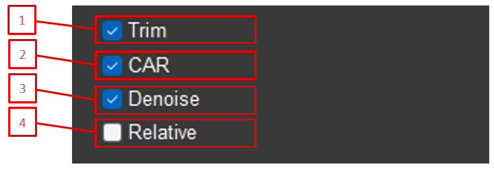
All application interfaces use a common signal-processing system. Each element of this system can be enabled or disabled separately and has its own settings. The transformations are applied in the following order:
Selection of data type (Type): RAW (raw data) or Filtered (pre-filtered in the 3–100 Hz range with a 50 Hz notch filter)
Trim: Removal of marked artifact segments
CAR (Common Average Reference): Re-referencing to a common reference electrode
Denoise (blink artifact suppression): Wavelet processing to remove blinks
Normalize: Amplitude normalization
IMF (Empirical Mode Decomposition): Decomposition into modes
Filter: Band-pass filtering
Epoch: Averaging over epochs
Power/Amplitude: Conversion to power or amplitude
1.2. Marking and Trim
1.2.1. Automatic Artifact Marking
Purpose: Automatic detection of signal segments with amplitude outliers.
How it works:
The signal is divided into 3-second windows.
The maximum and minimum are taken for each window.
Thresholds are calculated as doubled medians of these extrema: quantPl = 2*median(max), quantMn = 2*median(min)
Values outside the thresholds are clipped to the threshold values, reducing the impact of rare outliers.
Based on these thresholds, the system automatically marks artifact segments (in the Ignore field).
Marked segments are shown in yellow on the graph.
Physiological explanation:
The marking procedure is based on the idea of a “typical” amplitude range within 3-second windows: physiologically normal activity usually has a relatively stable amplitude, whereas sharp spikes are more often associated with artifacts. Clipping such spikes reduces their contribution to subsequent calculations while preserving the temporal structure of the signal.
1.2.2. Trim: Removing Marked Segments
Purpose: Removal of marked (yellow) artifact segments from the signal.
How it works:
Removal is performed when the Trim checkbox is enabled.
All segments marked as artifacts in the Ignore field are removed from the signal.
Time stamps for sections and comments are recalculated to account for the removed segments.
Signal time is recalculated as: Time = (1:sum(Ignore==0))/Fs
Use case: Used to exclude motion artifacts, blinks, electromagnetic interference, and other distortions.
Physiological explanation:
Artifacts are signals unrelated to the physiological activity of interest. For example:
Motion artifacts: When the participant moves their head, the electrodes shift relative to the skin, causing large voltage jumps.
Blink artifacts: The eyelid muscles generate electrical potentials during blinking, which are recorded by frontal electrodes.
Muscle artifacts: Tension in the neck or facial muscles creates high-frequency oscillations.
Artifact removal is necessary to obtain a “clean” signal that reflects only brain or cardiac activity.
1.3. CAR (Common Average Reference)
Purpose: Removal of common artifacts present in all channels.
Mathematical formula:
avgElectrodes = (F8 + AF4 + AF3 + F7) / 4 for each channel i: signal_i = signal_i - avgElectrodes
How it works:
The average value of the first four EEG electrodes (F8, AF4, AF3, F7) is calculated.
This average value is subtracted from each channel.
Components common to all channels are removed (for example, line noise and eye movements).
Use case: A standard EEG re-referencing method used to reduce the influence of common artifacts.
Physiological explanation:
EEG electrodes record the potential difference between an active electrode and a reference electrode. The problem is that the reference electrode itself (in the typical CleverPoint setup, usually at the center of the forehead or on the earlobe) may contain its own activity or artifacts.
CAR solves this problem:
Instead of a single reference electrode, the average of all electrodes is used.
This creates a “virtual” reference that reflects overall activity.
Components common to all electrodes (line noise, eye movements, general artifacts) are automatically subtracted.
Only the local activity of each electrode remains.
Analogy: Imagine measuring mountain heights relative to sea level. If sea level itself fluctuates, all measurements become distorted. CAR is like using the average level of all points for more accurate measurements.
1.4. Denoise (Blink Artifact Suppression)
Purpose: Removal of blink artifacts from the signal using wavelet processing.
Method: Wavelet denoising using the Daubechies 4 (db4) wavelet.
Parameters:
Decomposition level depends on the sampling frequency: Fs = 1000 Hz: N = 7 levelsFs = 500 Hz: N = 6 levelsOtherwise: N = 5 levels
Threshold processing with parameter alpha = 3
Level-dependent thresholding
How it works:
Wavelet decomposition of the signal into N levels
Determination of thresholds for each level based on coefficient statistics
Thresholding of the coefficients (removing small coefficients corresponding to noise)
Inverse wavelet transform
Noise is calculated as the difference: noise = original_signal - denoised_signal
Result: signal = original_signal - noise
Use case: Suppression of blink artifacts that distort EEG, especially in frontal channels.
Physiological explanation:
Blinks create short-term, large-amplitude artifacts due to eyelid muscle activity and eye movement. These artifacts have a characteristic shape and temporal structure, which makes it possible to isolate and attenuate them using wavelet transformation while preserving useful neural activity.
Why this matters: Blink artifacts mask weak but important EEG components (for example, the alpha rhythm in the 8–13 Hz range) and can create false changes in the spectrum.
1.5. Normalize
Purpose: Bring the signal amplitude to a standard level.
Formula: normalized_signal = 5 * signal / mean(abs(signal))
How it works:
The mean absolute value of the signal is calculated.
The signal is scaled so that the mean absolute value becomes 5.
Use case: Standardizing amplitudes to compare signals across participants or sessions.
Physiological explanation of normalization:
The amplitude of the EEG signal varies greatly between people and even between sessions for the same person. This depends on:
Skull and skin thickness
Quality of electrode contact
Individual characteristics of the brain
Level of activation
Why normalization is needed:
It makes it possible to compare signals between different people.
It removes the influence of technical factors (contact quality).
It focuses attention on patterns rather than absolute values.
It simplifies visualization (all signals are displayed on the same scale).
Important to understand:
Normalization does not change the shape of the signal, only its scale.
Relative changes are preserved.
Absolute values are lost (a normalized signal cannot be directly compared with a non-normalized one).
1.6. IMF (Empirical Mode Decomposition)
Purpose: Decompose the signal into intrinsic mode functions.
Method: EMD (Empirical Mode Decomposition) with a maximum of 5 modes.
How it works:
The signal is decomposed into intrinsic modes using the EMD algorithm.
The drop-down list contains 6 values:
IMF: no decomposition is applied; the signal remains unchanged
1: mode 1
2: mode 2
3: mode 3
4: mode 4
5: mode 5
If a specific mode is selected, only that mode is used: signal = imf(:, selected_mode)
Use cases:
Isolating specific frequency components
Removing baseline drift
Analyzing nonlinear and non-stationary processes
Physiological explanation of EMD:
Empirical Mode Decomposition is a method for decomposing a signal into “intrinsic modes” without using predefined basis functions (unlike the Fourier transform).
What modes are:
Modes are oscillatory signal components that have physical meaning.
Each mode has its own frequency and amplitude.
Modes adapt to the data (they are not fixed frequencies as in Fourier analysis).
Physiological meaning:
Mode 1 (high-frequency): the fastest components, possible noise
Modes 2–3: main rhythms (alpha, beta)
Mode 4: slower components, signal details
Mode 5 (low-frequency): slow changes, baseline drift, and possibly artifacts
Why use a specific mode:
Drift removal: Mode 5 often contains baseline drift (due to sweating or electrode movement).
Rhythm isolation: A specific mode may contain the rhythm of interest (for example, alpha).
Artifact removal: Some modes may contain artifacts that can be excluded.
Advantages of EMD:
Adaptivity: modes fit the signal
Nonlinearity: nonlinear processes can be analyzed
Non-stationarity: works with signals whose properties change over time
1.7. Filtering
Purpose: Isolate the signal in a specific frequency band.
Method: FIR filter (Finite Impulse Response) using the Parks–McClellan algorithm (firpm).
Filter parameters:
Transition band: ±0.5 Hz from the passband boundaries
Stopband attenuation: 80 dB
Filter order: calculated automatically
Filter types:
Type 0: No filtering
Type 1: Band-pass filter (single band)
Type 2: Ratio of two bands (band1 / band2)
Available ranges (Type 1):
Theta (4–8 Hz)
Theta1 (4–6 Hz)
Theta2 (6–8 Hz)
Alpha (8–13 Hz)
Alpha1 (8–10 Hz)
Alpha2 (10–13 Hz)
Beta (13–30 Hz)
Beta1 (13–20 Hz)
Beta2 (20–30 Hz)
Gamma (30–100 Hz)
Band ratios (Type 2):
Alpha/Theta (8–13 Hz / 4–8 Hz)
Alpha/Beta (8–13 Hz / 13–30 Hz)
Use case: Isolation of standard EEG bands, their sub-bands (theta1, theta2, alpha1, alpha2, beta1, beta2), and computation of band ratios.
Physiological explanation of frequency bands:
Delta (0.5–4 Hz):
Physiology: the slowest rhythms; associated with deep sleep (stages 3–4), coma, and pathological conditions
Neural mechanisms: synchronization of large cortical regions, reduced metabolism
When it appears: in adults, only during sleep; in infants, also during wakefulness (normal)
Clinical significance: excessive delta during wakefulness may indicate pathology
Theta (4–8 Hz):
Physiology: associated with light sleep, meditation, creative thinking, and learning
Neural mechanisms: synchronization of the hippocampus and cortex; important for memory consolidation
When it appears: with eyes closed, in relaxation, during REM sleep
Clinical significance: elevated theta may indicate drowsiness or pathology
Theta sub-bands:
Theta1 (4–6 Hz): slower theta, more often associated with drowsiness and transitional states
Theta2 (6–8 Hz): faster theta, more often associated with attention and cognitive processing
Alpha (8–13 Hz):
Physiology: the “resting rhythm”; dominant during relaxed wakefulness with eyes closed
Neural mechanisms: synchronization of occipital and parietal cortex; associated with the absence of visual stimulation
When it appears: with eyes closed, in a calm state; disappears when the eyes open or during mental effort
Clinical significance: absence of alpha may indicate pathology; alpha asymmetry between hemispheres may indicate problems
Alpha sub-bands:
Alpha1 (8–10 Hz): slower alpha, more often associated with relaxation and calmness
Alpha2 (10–13 Hz): faster alpha, more often reflects readiness for information processing
Beta (13–30 Hz):
Physiology: active wakefulness, attention, problem solving
Neural mechanisms: cortical desynchronization, active information processing
When it appears: with eyes open, during mental activity, movement
Clinical significance: increased beta may indicate stress, anxiety, and tension
Beta sub-bands:
Beta1 (13–20 Hz): associated with active thinking and attention
Beta2 (20–30 Hz): higher beta, more often associated with tension and stress
Gamma (30–100 Hz):
Physiology: high-level cognitive processing, binding information from different areas
Neural mechanisms: rapid synchronization of distant cortical regions; “binding” features into a unified perception
When it appears: during complex cognitive tasks, perception, and attention
Clinical significance: gamma activity abnormalities are associated with schizophrenia and autism
Band ratios (Type 2):
Alpha/Theta: an index of relaxation relative to drowsiness/slower processes
Alpha/Beta: an index of the balance between relaxation and cognitive activity
Why filtering is important:
The EEG signal contains all frequencies simultaneously. Filtering makes it possible to isolate the frequency range of interest and analyze it separately. For example, alpha activity is needed to study relaxation, while beta activity is used to study concentration.
1.8. Power vs Amplitude
Purpose: Convert the signal into power or amplitude.
Modes:
Amplitude: The original signal without change
Power: The signal squared: power = signal.^2
Physiological explanation of power:
Power equals the square of amplitude. It is a measure of the “energy” of activity.
Why power is important:
Amplitude may be positive or negative (the signal oscillates around zero).
Power is always positive and shows the “strength” of activity.
Power reflects overall activity better than amplitude.
Physiological meaning:
High alpha power: strong alpha activity = strong relaxation
High beta power: strong beta activity = strong cognitive activity
Low power: weak activity or artifacts
Comparison of modes:
Amplitude: Shows signal shape and the direction of change (positive/negative deflections)
Power: Shows the intensity of activity and does not depend on sign
When to use:
Amplitude: Signal visualization, waveform analysis, artifact detection
Power: Quantitative activity analysis, comparison between conditions, statistics
1.9. Epoch
Purpose: Average the signal using a sliding window.
Method: Sliding average using filtfilt (bidirectional filtering).
Interpretation: A heart rate variability metric that reflects parasympathetic activity. Higher values = greater variability = more relaxation.
Physiological explanation of RMSSD:
RMSSD measures short-term changes in RR intervals (beat to beat). It is one of the most sensitive indicators of parasympathetic (vagal) activity.
How the parasympathetic system works:
The vagus nerve sends signals to the heart.
These signals modulate heart rate depending on the phase of breathing.
During inhalation: pulse speeds up slightly.
During exhalation: pulse slows down slightly.
This creates the variability measured by RMSSD.
What the values mean:
High RMSSD (>50 ms in younger people): good parasympathetic activity, relaxation, recovery
Low RMSSD (<20 ms): reduced parasympathetic activity, stress, fatigue, possible health problems
Normal values depend on age (higher in younger people, lower in older people)
Why this matters:
RMSSD is a marker of the body’s ability to recover. Athletes with high RMSSD recover faster after exercise. Low RMSSD may indicate overtraining or chronic stress.
2.3.5. SDNN (Standard Deviation of NN Intervals)
Calculation method: SDNN = std(RR)
Interpretation: Overall heart rate variability. Reflects both sympathetic and parasympathetic activity.
Physiological explanation of SDNN:
SDNN is the standard deviation of all RR intervals. It is an integral measure of overall variability that reflects the functioning of the entire autonomic nervous system.
Sympathetic activity: may either increase variability (with moderate activation) or decrease it (under strong stress)
Circadian rhythms: variability changes throughout the day
Age: variability decreases with age
Clinical significance:
High SDNN (>100 ms in younger people): good autonomic regulation, good health
Low SDNN (<50 ms): reduced autonomic regulation, possible problems
SDNN <20 ms: very low variability, high risk of cardiovascular events
Comparison with RMSSD:
RMSSD is more sensitive to parasympathetic activity (short-term changes)
SDNN reflects total autonomic regulation (all changes)
Both parameters are important for a complete picture of ANS function
2.3.6. Functional Group (FG)
Calculation method:
SD1 and SD2 are calculated from the Poincaré plot.
Mean pulse is calculated.
The findFunctionalGroup_Z function is used, which:
normalizes SD1, SD2, and HR relative to age- and sex-specific norms (z-scores)
determines the functional group (0–13) based on the combination of z-scores
considers whether the section is a relaxation section (Calibration, Relax)
Physiological explanation of the functional group:
The functional group is a comprehensive assessment of the state of the autonomic nervous system based on normalization of HRV parameters relative to age- and sex-specific norms.
Interpretation: See the guide *Classification of Functional States*.
2.3.7. Concentration (CONCENT)
Calculation method:
The signal from electrode AF4 is filtered into three ranges:
Alpha (10–13 Hz)
Beta (20–30 Hz)
Gamma (30–90 Hz)
Envelopes are calculated using a 4-second window: envelope_alpha = filtfilt(moving_average, 1, abs(alpha_signal))envelope_beta = filtfilt(moving_average, 1, abs(beta_signal))envelope_gamma = filtfilt(moving_average, 1, abs(gamma_signal))
Concentration of attention is associated with activation of the prefrontal cortex and suppression of distracting signals. This is reflected in changes in the ratio of EEG frequency bands.
Neurophysiology of concentration:
Alpha activity (8–13 Hz): associated with relaxation and the absence of active processing
Beta activity (13–30 Hz): associated with active thinking and information processing
Gamma activity (30–90 Hz): associated with information binding and attentional focus
What this means:
During concentration: beta and gamma increase (active processing), alpha decreases (less relaxation)
During distraction: alpha may be high (relaxation), while beta and gamma are low (no active processing)
Interpretation of values:
Low values (<10): scattered attention, relaxation, possible drowsiness
Medium values (10–30): normal concentration
High values (>30): high concentration, active mental work, possibly tension
Why AF4 is used:
AF4 (right hemisphere, anterior frontal area) is used because this area is important for:
Attention control
Suppression of distracting stimuli
Working memory
Executive functions
2.3.8. Arousal (AROUSAL)
Calculation method:
Signals from AF3 and AF4 are filtered into alpha (8–13 Hz) and beta (13–30 Hz) ranges.
Power is calculated in an 8-second window: power_alpha = 1 + log10(sum(alpha_signal.^2) / window_length)power_beta = 1 + log10(sum(beta_signal.^2) / window_length)
Valence is the evaluation of an emotion as pleasant or unpleasant. Research shows that the left and right hemispheres process emotions differently.
Theory of hemispheric asymmetry (Davidson, 1992):
Left hemisphere (AF3):
processing of positive emotions
approach behavior
activity and enthusiasm
high alpha = low activation = relaxed but positively oriented state
Right hemisphere (AF4):
processing of negative emotions
withdrawal behavior
caution and anxiety
high alpha = low activation = relaxation, but with possible negative valence
Interpretation:
Positive values:
the right hemisphere is more relaxed (high alpha/beta)
the left hemisphere is more active (low alpha/beta)
positive emotions, pleasure, joy
Negative values:
the left hemisphere is more relaxed
the right hemisphere is more active
negative emotions, sadness, anxiety, discomfort
Close to zero: neutral emotions, balance
Important to understand:
Alpha activity is inversely related to cortical activation.
High alpha/beta = low cortical activation in that hemisphere.
Low alpha/beta = high cortical activation in that hemisphere.
The signal is influenced by tension in the forehead muscles.
Practical significance:
Persistently negative valence may indicate depression or anxiety.
Positive valence during relaxation is a good sign.
Changes in valence reflect emotional reactions to stimuli.
2.4. Data Export
The Export to CSV button saves all calculated parameters to a CSV file with delimiters, including:
Anthropometric data
Section time stamps
Section durations
EEG and ECG data validity (percent)
All frequency parameters by electrode
Brain activity parameters
Heart rhythm parameters
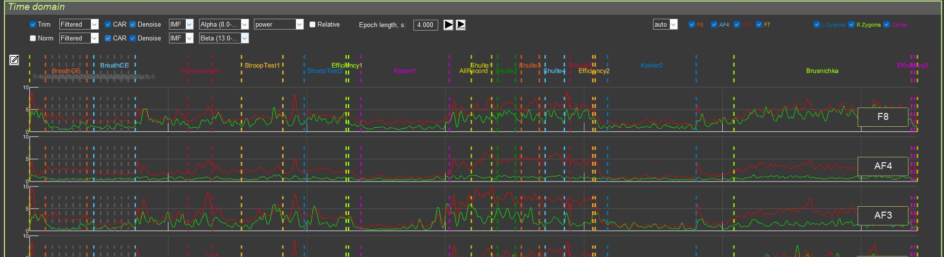
3. “Time Domain” Interface
3.1. Purpose
This interface is used for visualizing signals in the time domain, with the ability to overlay two different signal-processing pipelines.
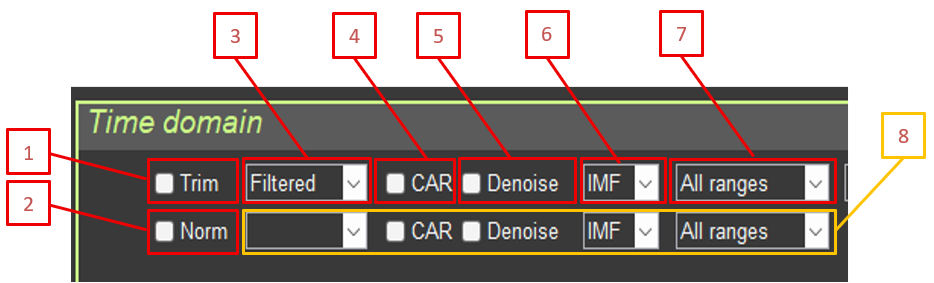
3.2. Controls
3.2.1. General Settings
Trim: Remove artifact segments
Norm (Normalize): Normalize amplitude
3.2.2. Signal Processing 1 (upper graph, green)
Type: RAW / Filtered (if no value is selected for signal 2, signal 2 is not shown)
CAR: Common average reference
Denoise: Blink artifact suppression
IMF: EMD mode selection
Filter: Frequency filter selection
Signal 2 controls: if no value is selected in Type for signal 2 (RAW / Filtered), signal 2 is not shown
3.2.3. Signal Processing 2 (lower graph, red)
The same parameters as for signal 1.
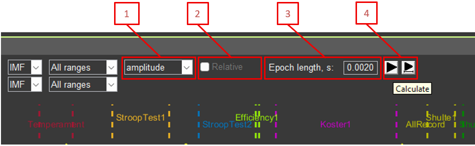
3.2.4. Additional Parameters
Amplitude/Power: Display amplitude or power
Relative: Relative or absolute values for signal power
Epoch length: Epoch length for averaging (in seconds)
Recalculation buttons (left button returns graph scaling to 100%; right button keeps the same signal fragment)
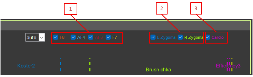
3.2.5. Electrode Selection
Checkboxes for showing or hiding the following channels:
F8, AF4, AF3, F7 (EEG)
L Zygoma, R Zygoma (EMG)
Cardio (ECG)
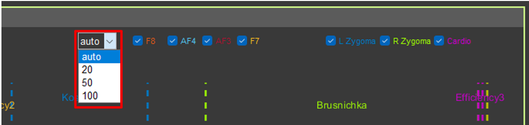
3.2.6. EEG Scale
Drop-down list for setting a fixed Y-axis scale for EEG channels (auto, 20, 50, 100 µV).
3.3. Signal Display
3.3.1. Graph Structure
Each channel is displayed on a separate axis.
All axes are synchronized in time (X-axis).
EEG channels are synchronized in amplitude (Y-axis).
3.3.2. Event Markers
Vertical colored lines indicate events and sections.
Different colors correspond to different sections.
Section names are displayed above the graphs.
Yellow dots indicate segments marked to be ignored.
3.3.3. Working with Sections
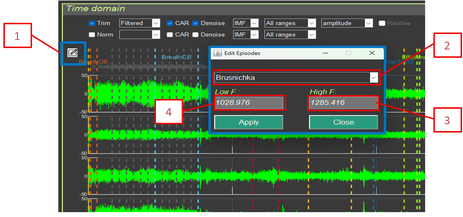
Edit episodes: Edit sections
Add Sector (-): Add a segment to ignore (select with the cursor)
Remove Sector (+): Remove a segment from the ignore list
Editing changes are not saved back into the source file, but they affect section markers in the exported data.
Edit episodes includes:
Section (episode) selection
Section (episode) start time for calculations
Section (episode) end time for calculations
3.4. Signal Transformations
All transformations are applied in the order described in Section 1. For each graph (1 and 2), an independent transformation chain can be specified, which allows different processing methods to be compared.
Example use case:
Graph 1: Filtered + CAR + Denoise (blink artifacts) + Alpha filter (8–13 Hz) + Power + Epoch length 4 s
Graph 2: Filtered + CAR + Denoise (blink artifacts) + Beta filter (13–30 Hz) + Power + Epoch length 4 s
This makes it possible to visually compare alpha and beta activity on one screen.
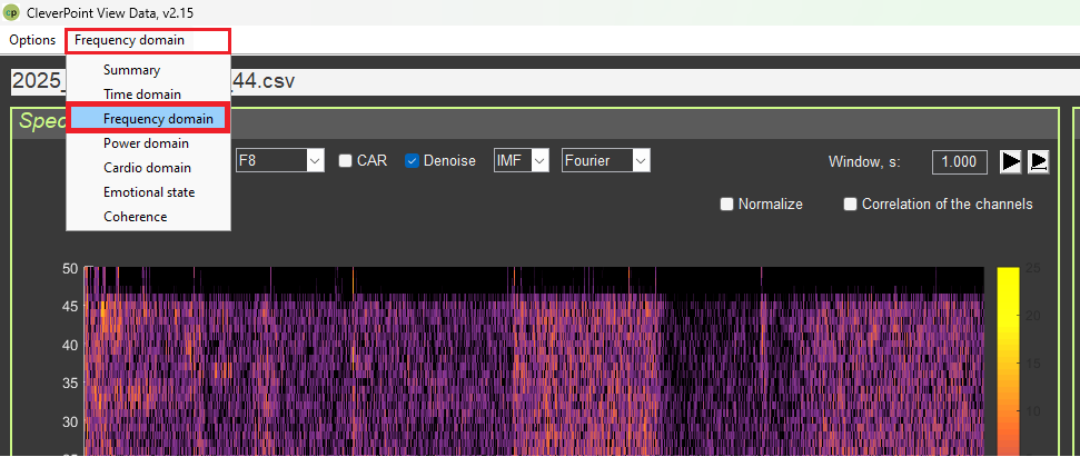
4. “Frequency Domain” Interface
4.1. Purpose
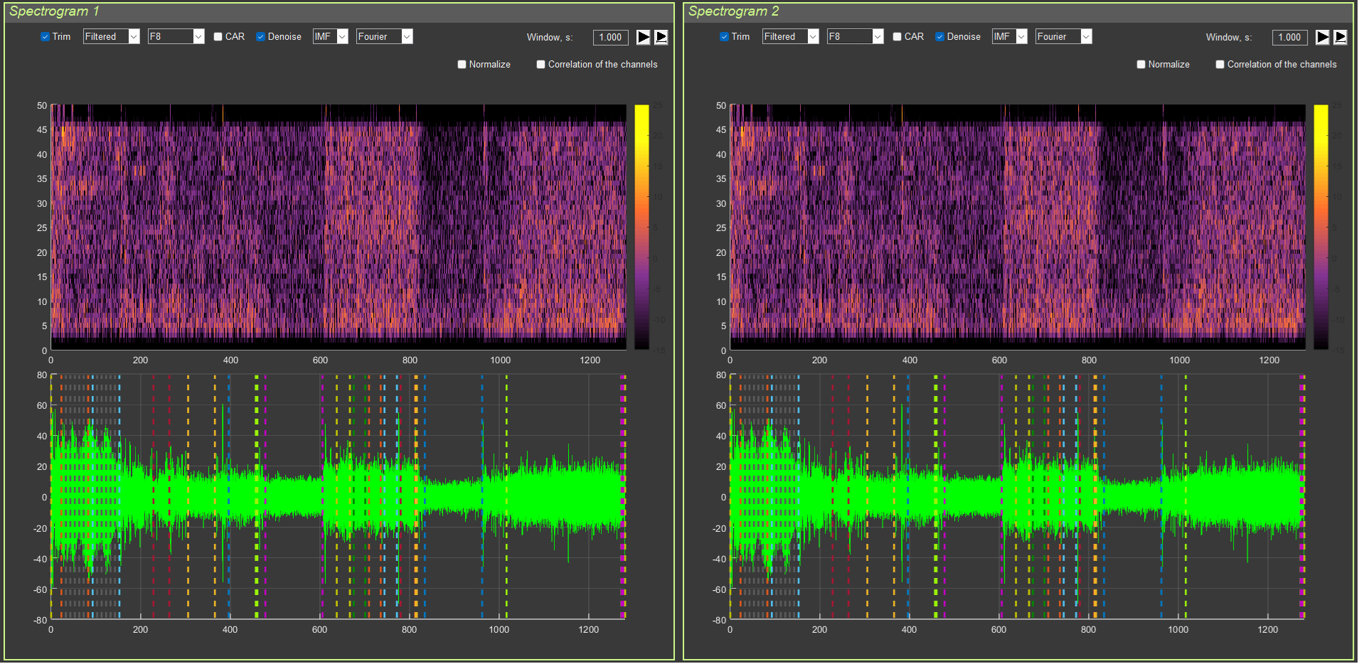
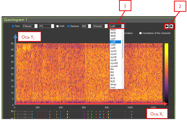
This interface is used for analyzing signals in the frequency domain by means of spectrograms (Short-Time Fourier Transform).
4.2. Interface Structure
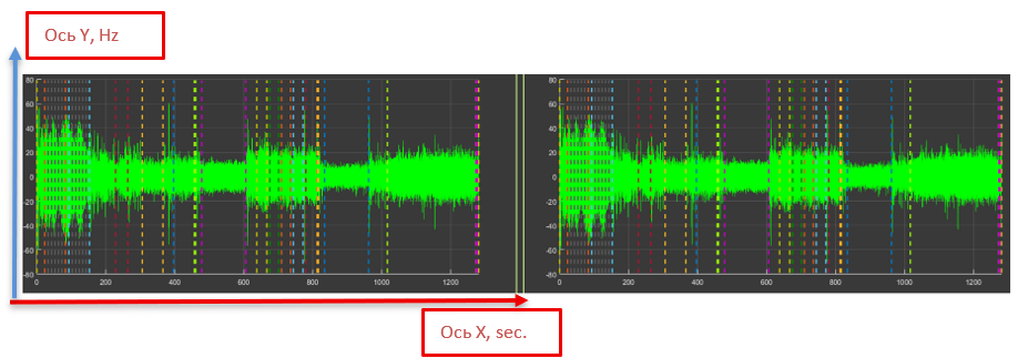
The interface is divided into two panels:
Spectrogram 1 (left panel)
Spectrogram 2 (right panel)
Each panel contains:
A spectrogram (upper graph)
A signal time series (lower graph)
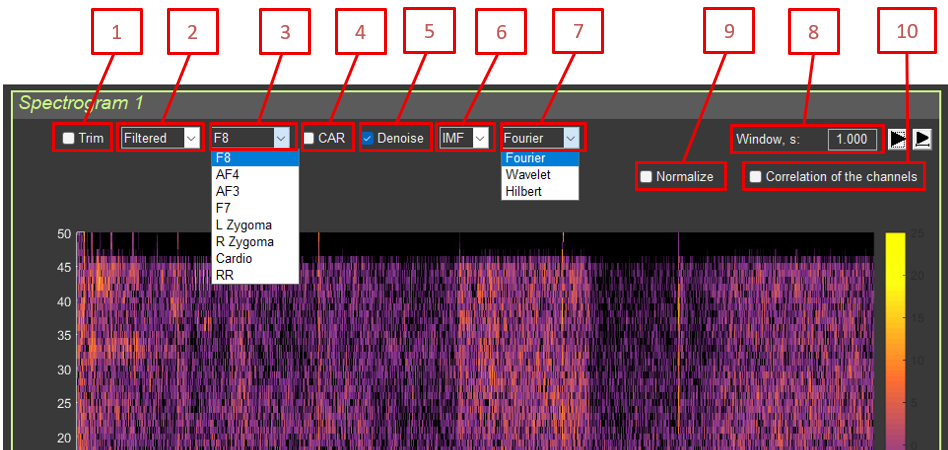
4.3. Controls
4.3.1. Signal Processing
Trim: Remove artifact segments
Type: Filtered / RAW
Channel: Select the channel (F8, AF4, AF3, F7, L Zygoma, R Zygoma, RR)
CAR: Common average reference
Denoise: Blink artifact suppression
IMF: EMD mode selection
Fourier/Wavelet/Hilbert: Spectral analysis method
Window, s: STFT window length (in seconds)
Normalize: Normalize the spectrogram
Correlation of the channels: Correlation between the channels in the two panels
Interpretation: Similar to STFT, but with better time resolution at high frequencies and better frequency resolution at low frequencies.
Advantages for EEG:
High frequencies (beta, gamma): short windows make it possible to determine the exact event time
Low frequencies (alpha, theta): long windows provide better frequency resolution
Physiological meaning:
Wavelet transformation uses windows of variable length—short windows for high frequencies and long windows for low frequencies. This corresponds well to the way the brain processes information.
Fast processes (for example, a response to a stimulus) require precise time resolution.
Slow rhythms (for example, alpha) require precise frequency resolution.
Wavelet transformation provides an optimal balance.
When to use:
For analyzing rapid events (responses to stimuli)
For analyzing slow rhythms with high precision
When both time and frequency resolution are needed simultaneously
Interpretation: Adaptive decomposition into intrinsic modes followed by analysis of instantaneous frequency. Suitable for nonlinear and non-stationary signals.
Physiological explanation of HHT:
The Hilbert–Huang Transform combines EMD (decomposition into modes) with instantaneous frequency analysis. This makes it possible to track how the frequency of a rhythm changes over time.
Physiological meaning:
The alpha rhythm frequency is not constant; it may “drift” from 8 to 13 Hz.
HHT shows these changes in instantaneous frequency.
This is important for understanding rhythm dynamics.
Advantages:
Adaptivity: adjusts to the signal
Nonlinearity: can process nonlinear phenomena
Instantaneous frequency: shows frequency changes over time
When to use:
For analyzing non-stationary signals (whose properties change over time)
For tracking rhythm frequency drift
For analyzing complex nonlinear processes
4.5. Channel Correlation
When the Correlation of the channels option is enabled:
A spectrogram is computed for the current channel in panel 1.
A spectrogram is computed for the selected channel in panel 2.
The cross-spectrum is computed: P_cross = (P1 .* conj(P2)).^0.7
Interpretation: Shows the synchrony of frequency components between two channels.
Physiological meaning:
Correlation between channels shows how synchronously two brain areas operate at specific frequencies. If two areas are synchronized at a certain frequency, they are “communicating” with each other. This may indicate a functional connection between the regions.
Different frequencies may have different degrees of synchrony:
Synchronization in alpha: the regions are relaxed together
Synchronization in beta: the regions are actively working together (for example, during problem solving)
Synchronization in gamma: rapid communication between regions; information binding
Practical significance:
Synchronization abnormalities may indicate connectivity problems.
Very high synchronization (>0.6) may indicate not only true connectivity, but also a common source contaminating the signal (noise or artifacts).
4.6. Time Series
The lower graph shows the original signal in the time domain with the same transformations (Trim, CAR, Denoise, IMF) as the spectrogram, but without frequency filtering. Denoise is used to suppress blink artifacts.
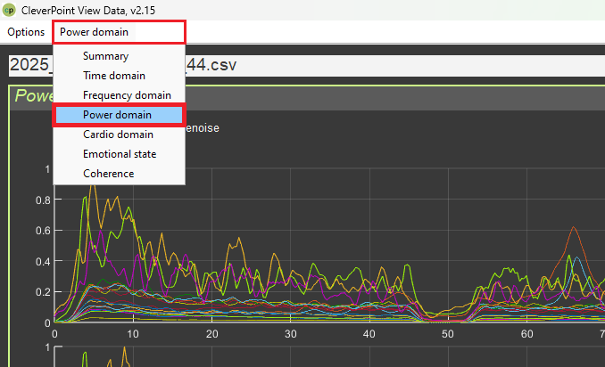
5. “Power Domain” Interface
5.1. Purpose
This interface is used to analyze signal power in frequency bands across recording sections. It has two modes:
Power by sections: a table of power values by section
Between-channel interactions: a graph of interactions between channels
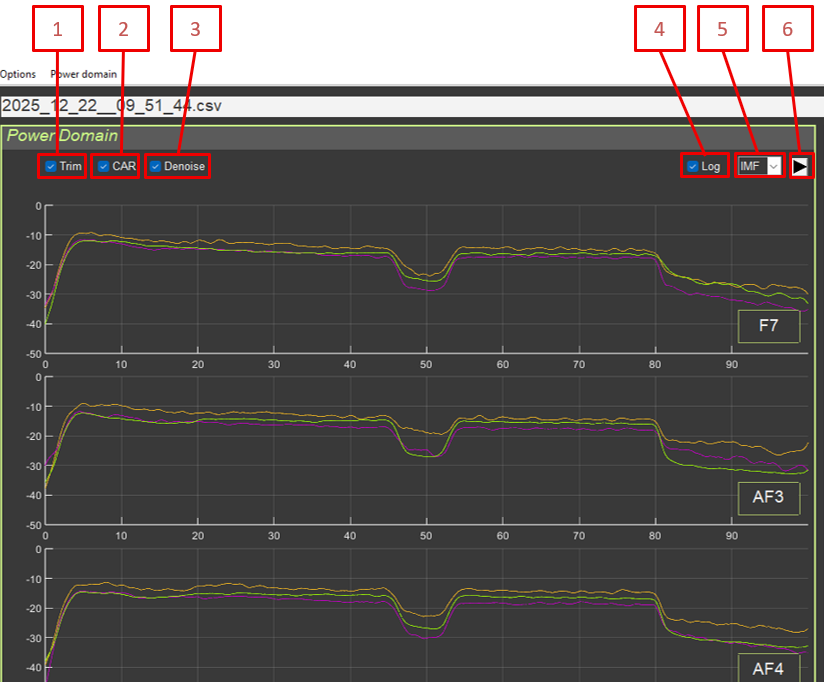
Common controls:
Trim: Remove artifact segments
CAR: Common average reference
Denoise: Blink artifact suppression
Log: Logarithmic scale
IMF: EMD mode selection
Recalculation button
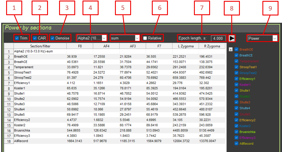
5.2. “Power by sections” Mode
5.2.1. Controls
Trim: Remove artifact segments
CAR: Common average reference
Denoise: Blink artifact suppression
Filter: Frequency filter selection
Function: Aggregation function (sum, mean, median, std)
Relative: Relative values (percentage of the total spectrum)
Epoch length: Epoch length for averaging
Recalculation button
Mode selection: Power by sections / Between-channel interactions
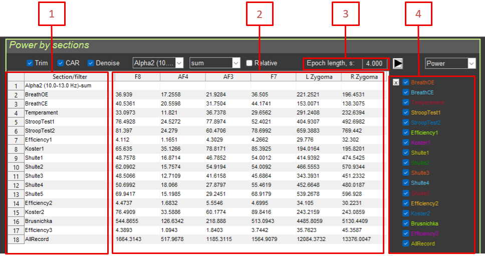
5.2.2. Results Table
The table contains:
Section/filter: Section name or filter name
F8, AF4, AF3, F7, L Zygoma: Power for each electrode
Epoch length: Epoch length
Power: Checkbox for including or excluding the section
5.2.3. Power Calculation Method
Transformations are applied: Trim, CAR, Denoise (blink artifacts)
The frequency filter is applied (if selected)
The signal is converted to power: power = signal.^2
Epoch averaging is applied: power_smoothed = filtfilt(moving_average, 1, power)
An aggregate statistic is calculated for each section: sum: sum(power_section) / Fs (power integral)mean: mean(power_section) (mean power)median: median(power_section) (median power)std: std(power_section) (standard deviation)
5.2.4. Relative Values
When Relative is enabled:
Total power (without filtering) is calculated for each channel.
Power in the selected band is expressed as a percentage: relative_power = 100 * filtered_power / total_power
Interpretation: Percentage of power in the selected frequency band relative to the total signal power.
Physiological explanation of relative power:
Absolute power depends on many factors (contact quality, individual characteristics). Relative power shows what share of total brain activity belongs to a given frequency band.
Relative power is more stable and makes it easier to compare people.
It shows the “balance” between different rhythms.
Examples:
Alpha 50%: half of the brain’s activity is alpha rhythm (strong relaxation)
Beta 30%: one third of the activity is beta rhythm (active thinking)
Theta 10%: one tenth of the activity is theta rhythm (light sleep or meditation)
Increased relative beta: transition toward active work
A change in balance reflects a change in functional state
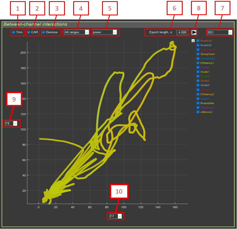
5.3. “Between-channel interactions” Mode
5.3.1. Purpose
Visualization of the relationship between two channels within a selected frequency band.
5.3.2. Controls
Trim: Remove artifact segments
CAR: Common average reference
Denoise: Blink artifact suppression
Filter: Frequency filter selection
Amplitude/Power: Amplitude or power
Epoch length: Epoch length
Mode selection: Power by sections / Between-channel interactions
Recalculation button
Electrode Y: Channel for the Y-axis
Electrode X: Channel for the X-axis
5.3.3. Calculation Method
Transformations and filtering are applied to each channel.
The signal is converted to amplitude or power.
Epoch averaging is applied.
For each section, a scatter plot is built: plot(X_channel, Y_channel)
5.3.4. Interpretation
Linear relationship: high correlation between channels
Clusters: different sections may form separate clusters
Cloud shape: reflects the type of interaction (synchronous, asynchronous, delayed)
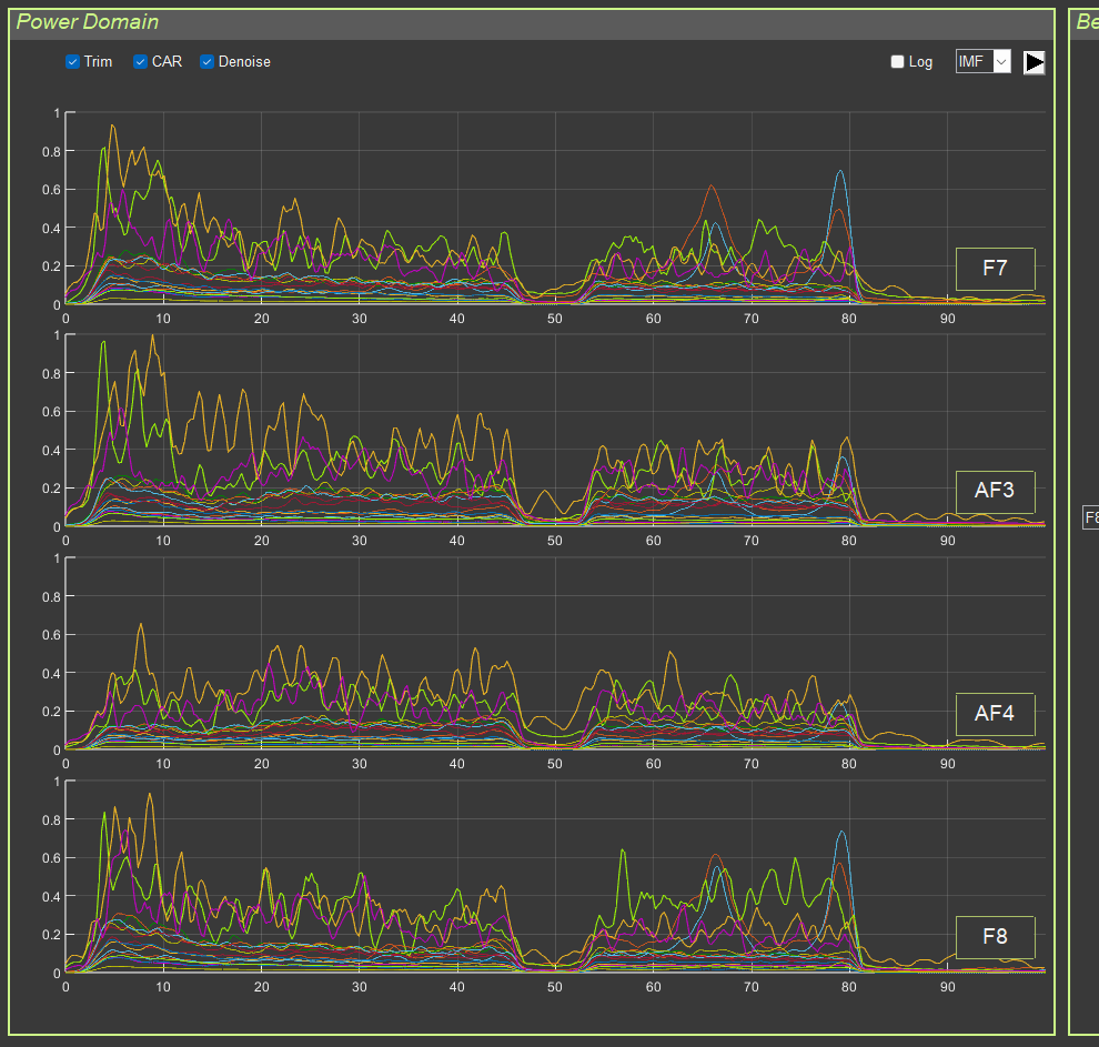
5.4. Frequency-Band Graphs
On the left side of the interface, power graphs for the four EEG channels (F7, AF3, AF4, F8) are displayed for all sections.
Method:
FFT is computed for each section.
A power spectrum is constructed: P = abs(FFT(signal)) / length(signal)
Smoothing is applied.
The spectrum from 0 to 100 Hz is displayed.
Colors: each section has its own color for visual distinction.
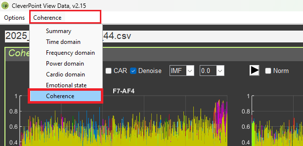
6. “Coherence” Interface
6.1. Purpose
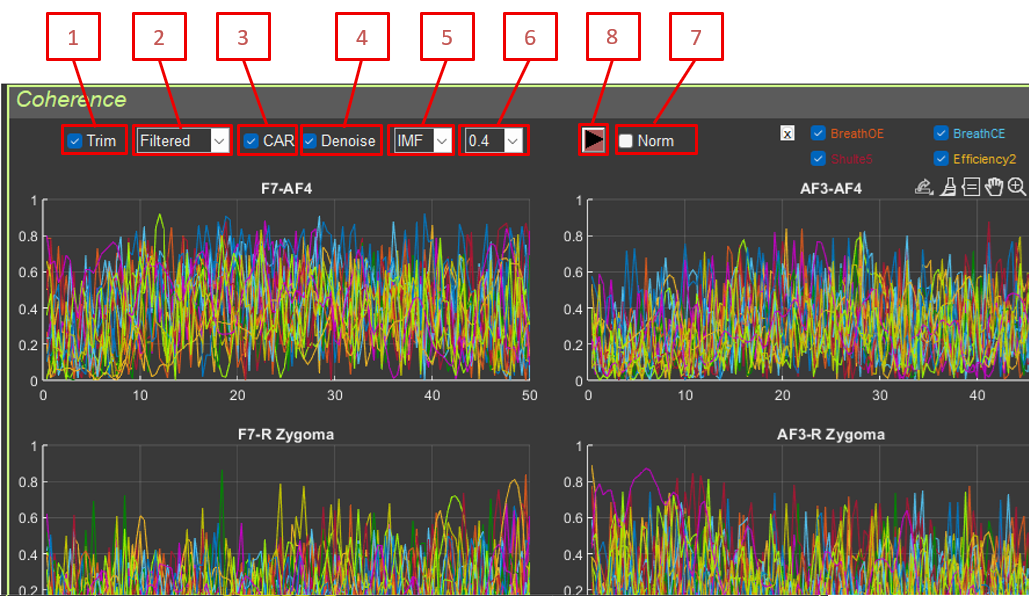
This interface is used to analyze coherence between pairs of EEG electrodes. Coherence shows the degree of synchrony of frequency components between two channels.
6.2. Controls
Trim: Remove artifact segments
Type: RAW / Filtered
CAR: Common average reference
Denoise: Blink artifact suppression
IMF: EMD mode selection
df: Frequency resolution (0.0, 0.2, 0.4, 0.6, 0.8, 1.0 Hz)
Norm: Normalize coherence
Recalculation button
6.3. Coherence Calculation Method
Formula: the mscohere (Magnitude Squared Coherence) function is used: [Cxy, F] = mscohere(signal1, signal2, [], [], frequencies, Fs)
Parameters:
signal1, signal2: signals from two electrodes after processing
frequencies: frequency vector for calculation (from df to 50 Hz with step df)
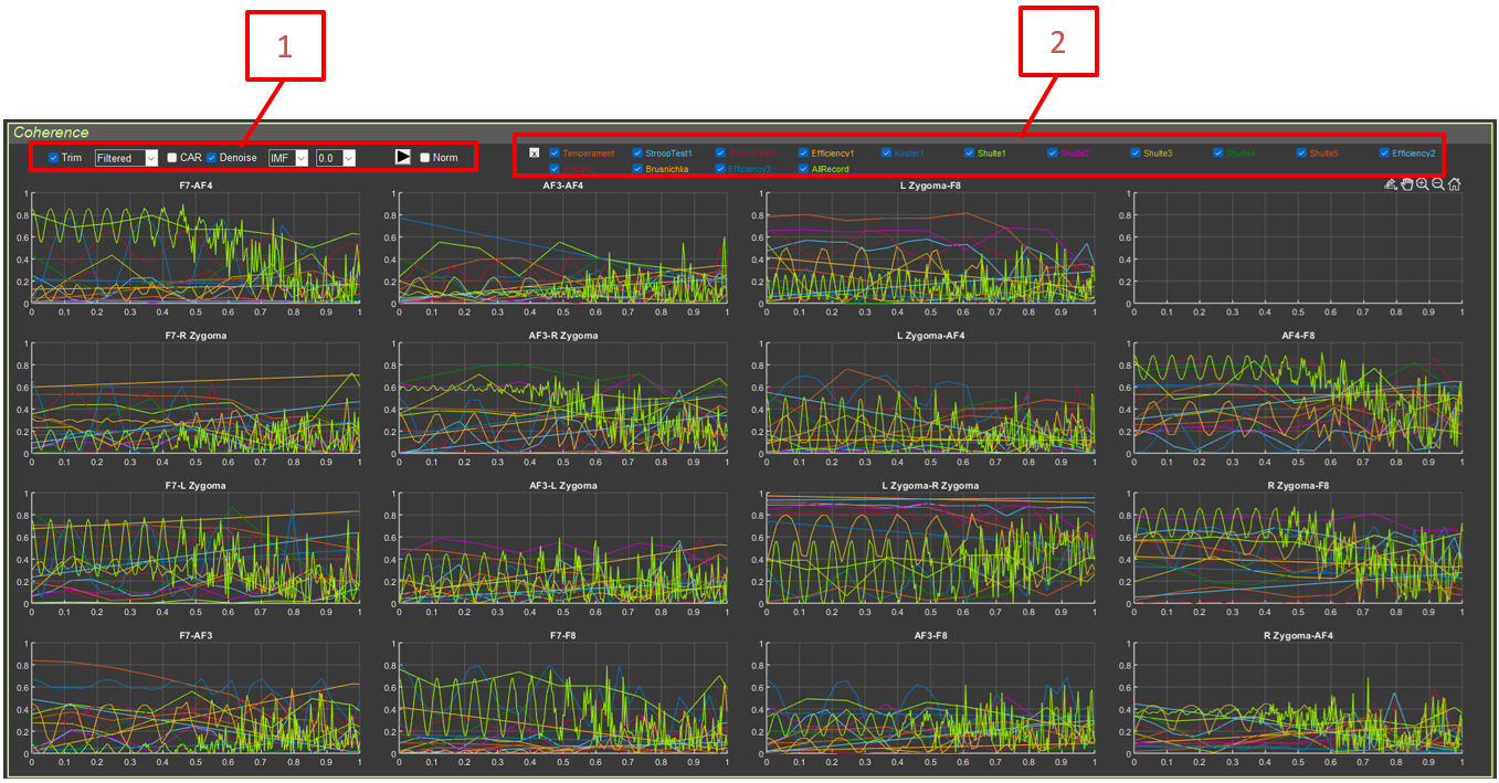
The interface contains a 16-plot grid (4 × 4), where each cell corresponds to a pair of electrodes:
F8–AF4, F8–AF3, F8–F7
AF4–AF3, AF4–F7
AF3–F7
For each pair, coherence curves are shown for all sections, and each section has its own color.
Controls:
Power: Checkbox for including or excluding sections
6.5. Interpretation
Physiological explanation of coherence:
Coherence measures how synchronously two brain areas operate at a specific frequency.
High coherence (close to 1):
Synchronous activity between channels
Functional connection between brain regions
Possible synchronization of neural ensembles
Possible common noise source (interference, muscle artifacts)
Low coherence (close to 0):
Independent channel activity
No functional connection
Frequency specificity:
Coherence can be high in some frequency ranges and low in others.
This reflects frequency-specific functional connections.
Frequency-specific relationships:
Alpha coherence (8–13 Hz): associated with relaxation and resting synchrony
Beta coherence (13–30 Hz): associated with active information processing and cognitive tasks
Gamma coherence (30–100 Hz): associated with information binding and perception
Practical significance:
Changes in coherence reflect changes in functional brain networks.
High coherence in appropriate ranges is a sign of efficient brain functioning.
6.6. Use in Research
Analysis of functional brain connectivity
Study of synchronization between regions
Diagnosis of connectivity abnormalities
Monitoring of connectivity changes over time
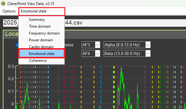
7. “Emotional State” Interface
7.1. Purpose
This interface is used to analyze emotional state based on EEG signals. It uses the Valence–Arousal model.
7.2. Interface Structure
The interface is divided into two panels:
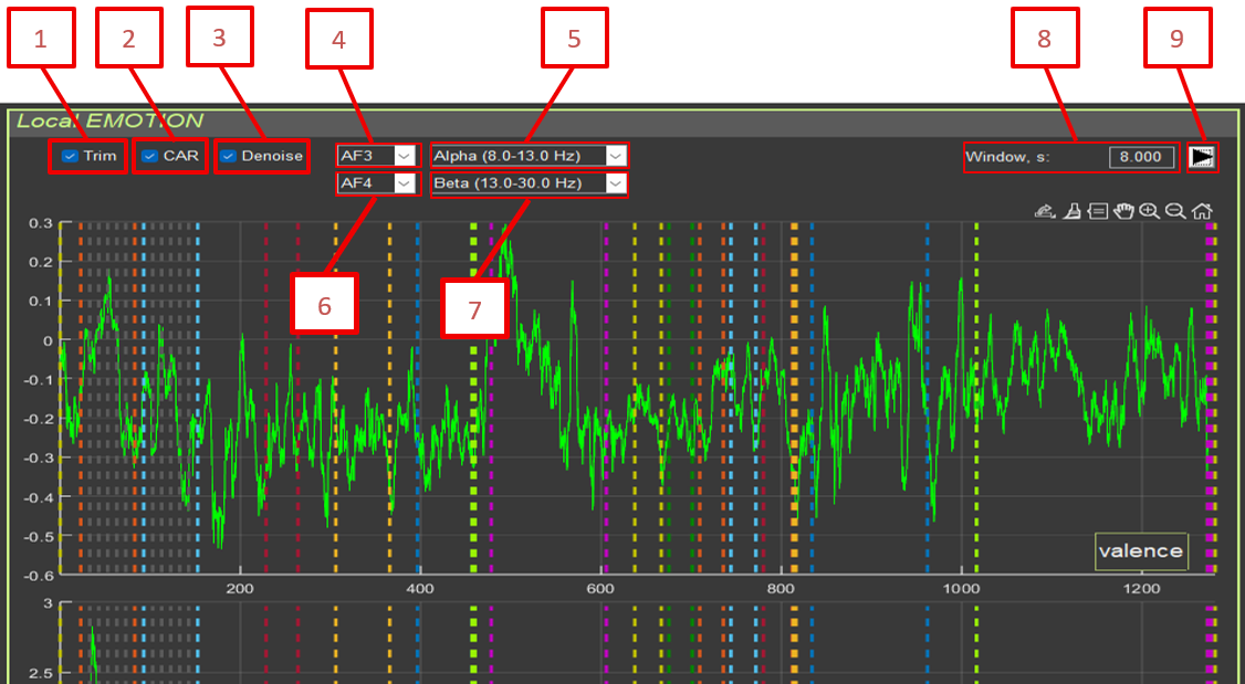
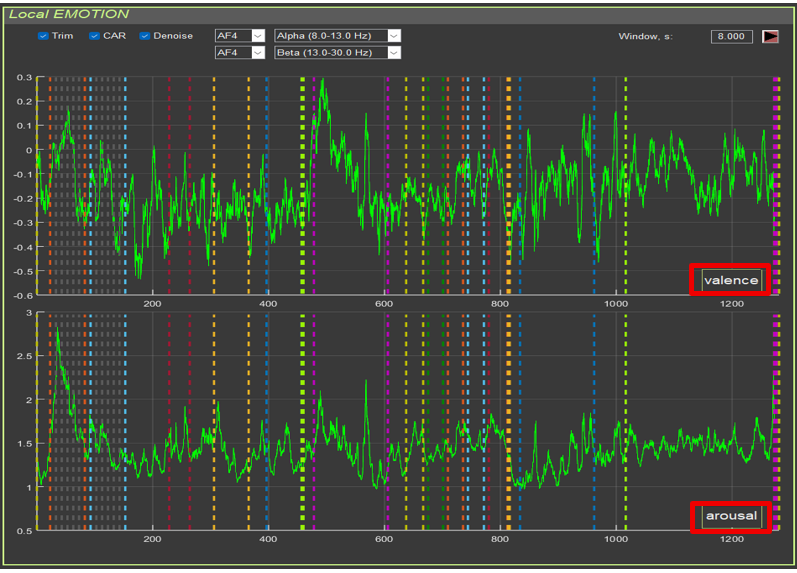
Local EMOTION: time series of valence and arousal
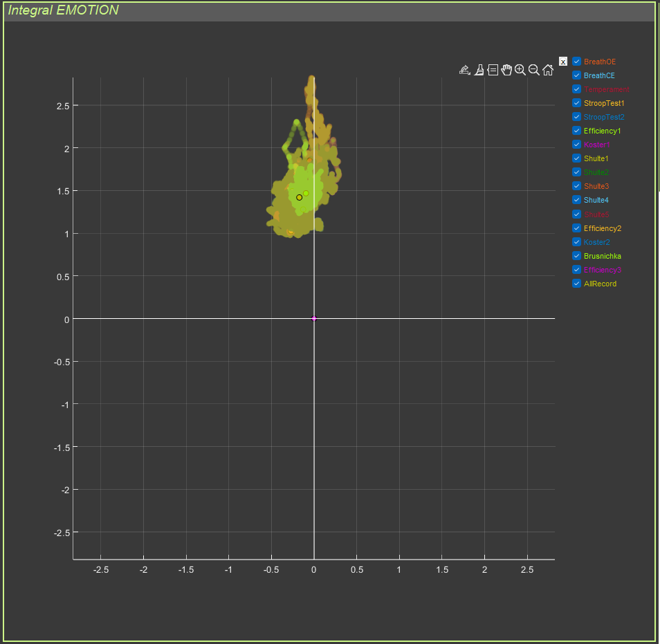
Integral EMOTION: integral emotion map (scatter plot)
7.3. Controls
7.3.1. Signal Processing
Trim: Remove artifact segments
CAR: Common reference processing
Denoise: Blink artifact suppression
Electrode 1: First electrode (default: AF3)
Filter 1: Frequency filter for the first electrode (default: Alpha 8–13 Hz)
Electrode 2: Second electrode (default: AF4)
Filter 2: Frequency filter for the second electrode (default: Beta 13–30 Hz)
Window, s: Window length for power calculation (default: 8 seconds)
Recalculation button
7.4. Emotion Calculation Method
7.4.1. Power Computation
For each electrode and frequency band:
Filtering in the selected band is applied.
Power is computed in a sliding window: window_samples = window_seconds * Fsfor i = 1:(length(signal) - window_samples) power(i) = 1 + log10(sum(signal(i:i+window_samples-1).^2) / window_samples)end
Power formula: power = 1 + log10(mean(signal_window.^2))
Theoretical rationale: The beta/alpha ratio reflects the activation level of the cerebral cortex. Beta activity is associated with active thinking and stress, while alpha activity is associated with relaxation.
Physiological explanation of arousal:
Arousal is the general activation level of the nervous system, ranging from deep sleep to severe stress.
Neurophysiology of arousal:
Low arousal: alpha rhythm dominates (8–13 Hz)
relaxed wakefulness
eyes closed
meditation
calm state
Medium arousal: mixed activity
eyes open
normal activity
alpha/beta balance
High arousal: beta rhythm dominates (13–30 Hz)
active thinking
problem solving
stress
anxiety
physical activity
Interpretation:
Low values (<0.5): low arousal, relaxation, possible drowsiness
Medium values (0.5–1.5): normal arousal, wakefulness
High values (>1.5): high arousal, stress, active mental work
Clinical significance:
Persistently high arousal may indicate chronic stress or anxiety.
Very low arousal may indicate depression, fatigue, or drowsiness.
Optimal arousal depends on the task (low for rest, medium to high for work).
Theoretical rationale: Alpha/beta asymmetry between the left and right hemispheres reflects emotional valence. The left hemisphere (AF3) is associated with positive emotions; the right hemisphere (AF4) with negative emotions.
Physiological explanation of valence:
Valence is the evaluation of an emotion as pleasant or unpleasant. Research shows that the left and right hemispheres process emotions differently.
Theory of hemispheric asymmetry (Davidson, 1992):
Left hemisphere (AF3):
processing of positive emotions
approach behavior
activity, enthusiasm
high alpha = low activation = relaxed state with a positive emotional orientation
Right hemisphere (AF4):
processing of negative emotions
withdrawal behavior
caution, anxiety
high alpha = low activation = relaxation, but with possible negative valence
Interpretation:
Positive values:
the right hemisphere is more relaxed (high alpha/beta)
the left hemisphere is more active (low alpha/beta)
positive emotions, pleasure, joy
Negative values:
the left hemisphere is more relaxed
the right hemisphere is more active
negative emotions, sadness, anxiety, discomfort
Close to zero: neutral emotions, balance
Important to understand:
Alpha activity is inversely proportional to cortical activation.
High alpha/beta = low cortical activation in that hemisphere.
Low alpha/beta = high cortical activation in that hemisphere.
Practical significance:
Positive valence during relaxation is a good sign.
Changes in valence reflect emotional responses to stimuli.
7.4.4. Outlier Handling
Values are clipped at the 95th percentile to remove artifact outliers: quantile_arousal = quantile(abs(arousal), 0.95)arousal(abs(arousal) > quantile_arousal) = sign(arousal) * quantile_arousal
The same is done for valence.
7.5. Display
7.5.1. Local EMOTION
Two graphs:
Arousal: arousal time series (green line)
Valence: valence time series (green line)
Both graphs are synchronized in time and contain section markers.
7.5.2. Integral EMOTION
Scatter plot:
X-axis: Valence
Y-axis: Arousal
Points: each point represents one moment in time
Colors: different sections have different colors
Large points: median values for each section
Emotion quadrants:
Upper right (high valence, high arousal): joy, enthusiasm
Upper left (low valence, high arousal): anxiety, anger
Lower left (low valence, low arousal): sadness, depression
Lower right (high valence, low arousal): calmness, satisfaction
Physiological explanation of the emotion quadrants:
Upper right quadrant (High valence + High arousal):
Emotions: joy, enthusiasm, excitement, delight
Physiology:
activation of the left hemisphere (positive emotions)
high beta activity (active thinking)
increased sympathetic activity, but in a positive context
activation of the left hemisphere (positive emotions)
high alpha activity (relaxation)
low beta activity (absence of stress)
high parasympathetic activity
balanced autonomic nervous system
Behavior: rest, recovery, positive relaxation
Important:
The quadrants are conditional and show not absolute emotions, but changes in emotion:
left to right: from less positive to more positive (or less negative)
bottom to top: from weaker to stronger
Emotion dynamics:
Emotions are not static; points may move between quadrants.
Transitions reflect changes in emotional state.
A healthy person may appear in different quadrants depending on the situation.
A problem may exist if a person remains in one quadrant continuously, especially a negative one.
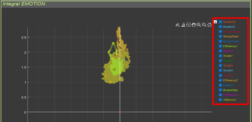
7.6. Section Selection
Checkboxes to the right of the scatter plot make it possible to include or exclude sections from the display. This is useful for comparing emotional states across conditions.
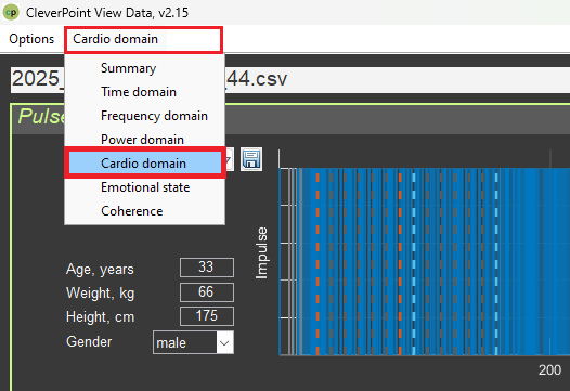
8. “Cardio Domain” Interface
8.1. Purpose
This interface is used for comprehensive analysis of heart rate variability (HRV) based on the ECG signal.
8.2. Interface Structure
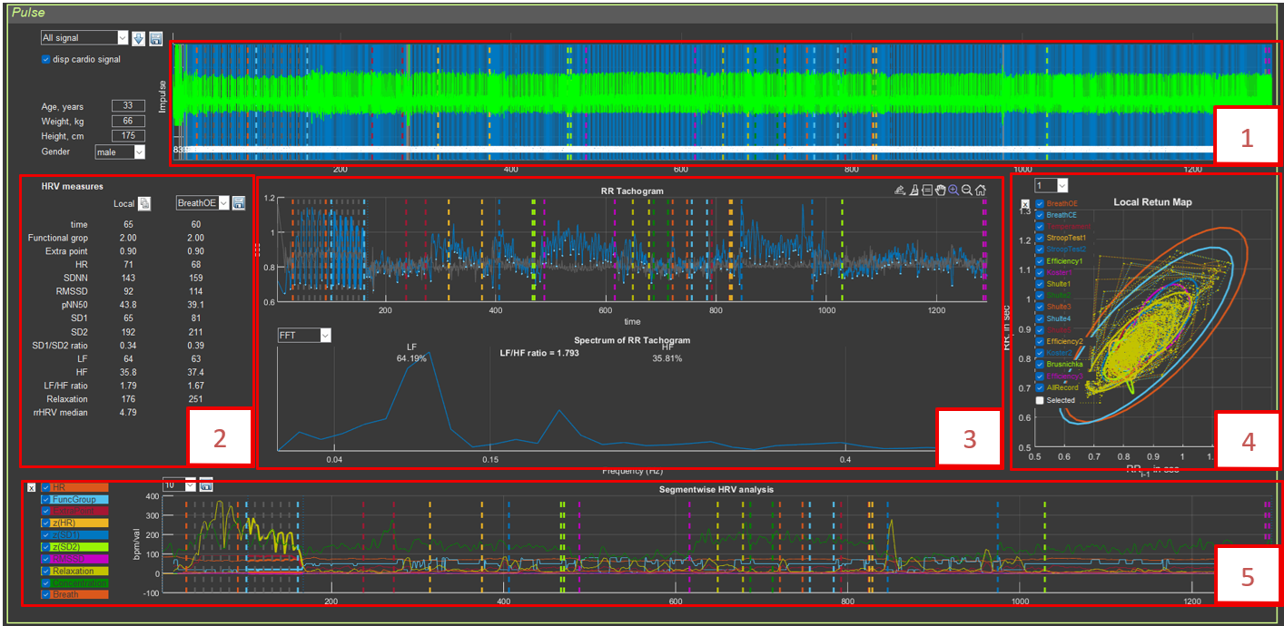
The interface contains:
Top panel: visualization of pulses and RR intervals
Middle left panel: HRV parameter table
Middle center panel: RR tachogram and spectrum
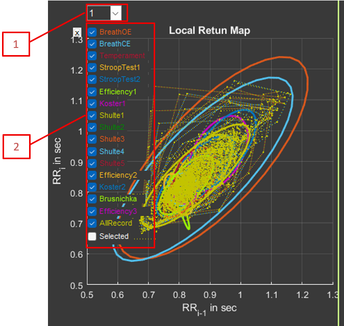
Middle right panel: Poincaré plot (Local Return Map)
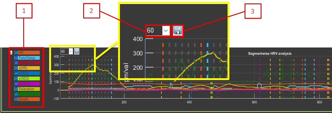
Bottom panel: segmental HRV analysis
8.3. Controls
8.3.1. General Settings
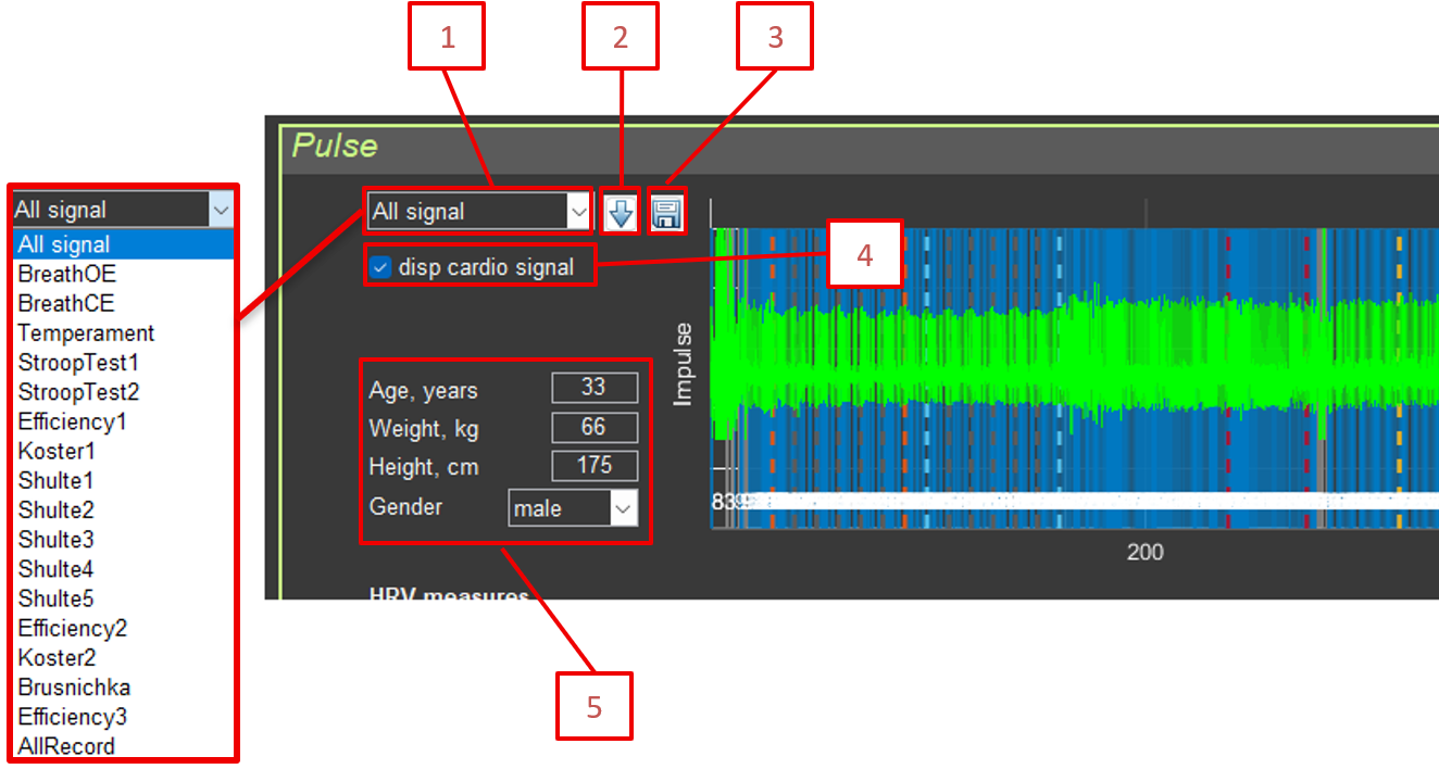
Sector: Select the section for analysis (All signal or a specific section)
Calculate HRV measures: Button for recalculating HRV metrics on the ECG segment selected in Sector
Save RR: Save RR intervals to CSV
disp cardio signal: Display the original ECG signal
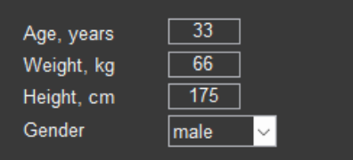
Age, Weight, Height, Gender: Anthropometric data (used for normalization)
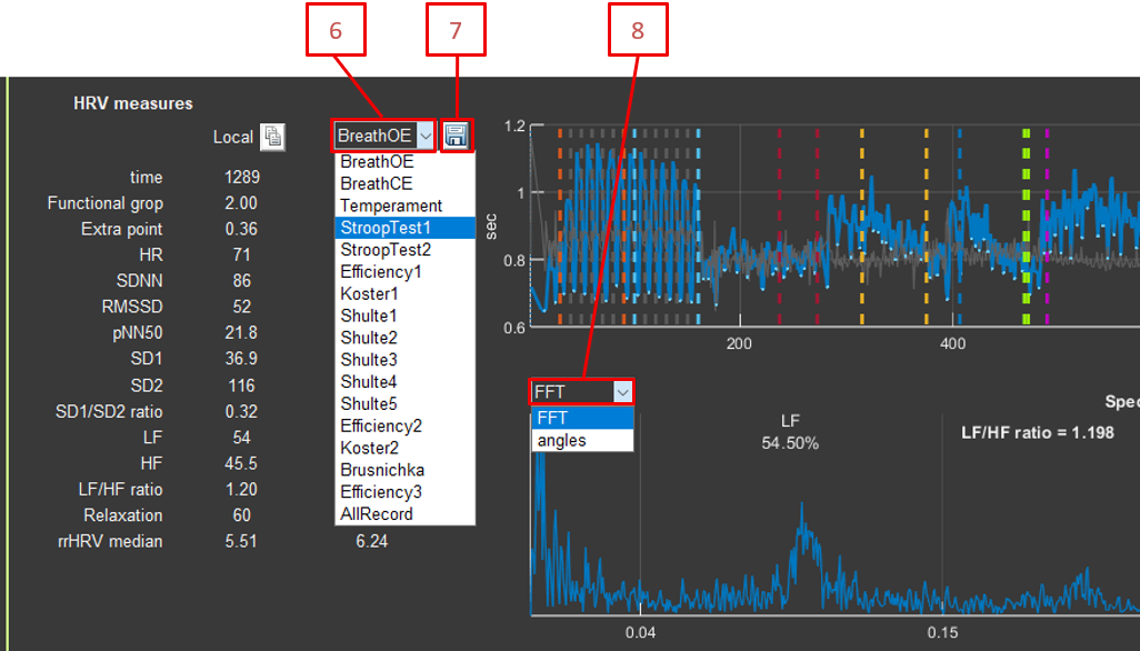
Sector: Select the section for analysis (AllRecord or a specific section)
Save HRV: Save HRV parameters by section to CSV
FFT type:FFT or Angles (angles in the Poincaré plot)
Shift RR: Shift for the Poincaré plot (1–15 intervals)
Average Window: Averaging window for segmental analysis (10–100 intervals)
Physiology: balance between sympathetic and parasympathetic systems
Interpretation:
High LF/HF (>2): predominance of sympathetic activity, stress, activation
Low LF/HF (<1): predominance of parasympathetic activity, relaxation, rest
Normal LF/HF (1–2): balanced state
Normalized units (nu):
LF_nu and HF_nu express the percentage of total power excluding VLF.
This allows comparisons between people by removing the influence of total power.
LF_nu + HF_nu = 100%
Clinical significance:
Reduced HF and increased LF/HF are markers of stress and fatigue.
Athletes at rest often show high HF and low LF/HF.
Under chronic stress, LF/HF is persistently elevated.
Recovery after exercise is accompanied by an increase in HF.
8.5.4. Functional Group
Interpretation: Functional state of the autonomic nervous system.
Physiological explanation of the functional group:
The functional group is a comprehensive evaluation of autonomic nervous system state based on normalization of HRV parameters relative to age- and sex-specific norms.
How it works:
Each person has “normal” SD1, SD2, and HR values based on age and sex.
Actual values are compared with these norms (z-scores).
The combination of z-scores determines the functional group.
See the document *Classification of Functional Groups*.
rrHRV median:
Median distance to the central point on the map of relative RR intervals.
Extra point:
Additional score in the functional group (0–100).
8.6. Visualization
8.6.1. RR Tachogram
Graph of RR intervals over time:
Blue line: RR intervals
Gray points: local minima (respiratory cycles)
Green line: signal power (scaled)
Gray vertical lines: section markers
8.6.2. RR Tachogram Spectrum
FFT spectrum of the interpolated RR signal:
X-axis: frequency (0–0.5 Hz)
Y-axis: spectral amplitude
LF (0.04–0.15 Hz) and HF (0.15–0.4 Hz) ranges are marked
LF%, HF%, and LF/HF ratio are displayed
8.6.3. Poincaré Plot (Local Return Map)
Scatter plot of RR(i) versus RR(i-1) or RR(i-shift):
Each point: a pair of consecutive RR intervals
Colors: different sections
Ellipses: 2SD1 and 2SD2 for each section
Shift RR: shift for the Poincaré plot (1–15 intervals)
Checkboxes for including or excluding sections
Physiological explanation of the Poincaré plot:
The Poincaré plot (return map) is a graphical way to visualize heart rate variability by showing the patterns of RR interval changes.
How to read the plot:
Each point = a pair of consecutive RR intervals
X-axis: RR(i-1), the previous interval
Y-axis: RR(i), the current interval
If the heart beat like a metronome, all points would be in one place.
Typical shapes:
Round/oval shape (healthy heart):
high variability
good adaptability
healthy ANS state
SD1 and SD2 are roughly equal
Elongated shape along the diagonal:
low short-term variability (small SD1)
long-term trends remain (larger SD2)
possible stress or fatigue
low SD1/SD2
Compact cloud:
low variability overall
very regular heartbeat
possible health problems
both SD1 and SD2 are small
Shifted center:
change in mean RR
transition between states (rest → load)
response to a stimulus
Physiological meaning of SD1 and SD2:
SD1 (minor axis):
short-term variability
beat-to-beat changes
predominantly parasympathetic activity
associated with respiratory arrhythmia
SD2 (major axis):
long-term variability
trends and slow changes
sympathetic + parasympathetic activity
associated with the baroreflex and other slow regulatory processes
Clinical significance:
Healthy people: round or oval cloud, SD1/SD2 ≈ 0.3–0.5
Stress: the cloud becomes elongated, SD1 decreases
Aging: the cloud becomes more compact, both SDs decrease
Pathology: a very compact cloud or an unusual shape
8.6.4. Segmental HRV Analysis
The graph shows the dynamics of HRV parameters over time:
HR: heart rate
FuncGroup: functional group (×10)
ExtraPoint: additional score (×100)
z(HR): pulse z-score
z(SD1): SD1 z-score
z(SD2): SD2 z-score
RMSSD: RMSSD
Relaxation: Relaxation
Concentration: Concentration (from EEG)
Breath: breathing rate
All parameters are calculated in a sliding window with 75% overlap.
Checkboxes for including or excluding HRV parameters
Average Window: Averaging window for segmental analysis (10–100 intervals)
Save continuously HRV: Save continuous HRV parameters over time
8.7. Data Export
Save HRV: Save HRV parameters by section to CSV
Save RR: Save RR intervals to CSV
Save continuously HRV: Save continuous HRV parameters over time
9. Conclusion
Conclusion
CleverPoint View provides a comprehensive set of tools for physiological signal analysis with detailed control over every processing stage. Understanding how each transformation works helps researchers to:
Interpret results correctly: Knowledge of the mathematical foundations of the methods helps avoid incorrect conclusions.
Choose optimal parameters: Understanding the effect of each parameter on the result makes it possible to adjust the analysis to a specific task.
Validate results: Knowledge of the limitations of methods helps assess result reliability.
Publish results: A detailed description of processing methods is required for scientific publications.
9.1. Recommendations for Use
Always document processing parameters: record all settings used (Trim, CAR, Denoise, filters, etc.), including a note about blink artifacts.
Check data quality: use the Time domain interface to visually inspect signals before analysis.
Compare different methods: use the option to overlay two processing pipelines.
Account for anthropometric data: for HRV analysis, always specify age, sex, height, and weight.
Validate results: compare results with literature data and known norms.
9.2. Additional Resources
Official website: cleverpoint.pro
Application version: 2.15
Supported formats: CSV with section metadata
Note: This guide is based on CleverPoint View Data version 2.15. All described methods and formulas correspond to the implementation in the application code.
9.3. Beginner’s Guide
If you are new to electrophysiology, we recommend the following order of study:
1. Start with the basics (Section 0):
Learn what EEG, ECG, and EMG are.
Understand the meaning of frequency ranges (alpha, beta, theta, gamma).
Learn about the autonomic nervous system and HRV.
2. Study signal processing (Section 1):
Understand why each operation is needed (Trim, CAR, Denoise, etc.), especially Denoise for blinks.
Start with simple operations (Trim, Filter).
Gradually add more complex ones (CAR, Denoise, EMD), where Denoise is responsible for blink artifacts.
3. Practice with the interfaces:
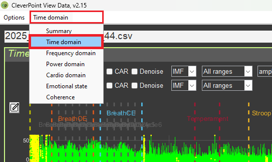
Time domain: start here—signal visualization will help you understand what is happening.
Summary: use it for an overview—you will see all parameters at once.
Frequency domain: study spectrograms—you will understand frequency patterns.
Cardio domain: study HRV—an important indicator of health.
Emotional state: study emotions—an interesting application of EEG.
4. Interpret results:
Always consider the physiological meaning of parameters.
Compare with normal values.
Take context into account (rest vs. load).
Do not rush to conclusions—one parameter does not provide the full picture.
5. Study the literature:
Read scientific papers on psychophysiology.
Learn the normal values of parameters.
Understand the limitations of the methods.
Important to remember:
Electrophysiology is a complex science that requires time to learn.
Not all parameters can always be interpreted unambiguously.
Context is very important—the same values may mean different things in different situations.
Always critically evaluate results and compare them with the literature.